qnetworks—a Queueing Networks analysis package for GNU Octave

About qnetworks

qnetworks is a Queueing Networks analysis package written in GNU Octave. It includes implementations of some QN algorithms. At the moment, the following algorithms are available:

• Exact analysis of single or multi-class, product-form open Queueing Networks (Jackson networks or BCMP networks).
• Mean Value Analysis (MVA) for single or multi-class closed networks.
• MVA for multiclass, mixed (open/closed) networks.
• Approximate MVA for closed, multi-class QN, using Bard-Schweitzer approximation.
• The convolution algorithm for closed, single-class product-form networks.
• MVABLO for closed, single-class QN with blocking.
• Computation of Asymptotic, Balanced System and Geometric bounds.
• Transient as well as steady-state analysis of Markov chains (computation of sojourn times and expected time to absorption for continuous-time Markov chains).
• Analysis of the following single-station queueing systems: M/M/1, M/M/m, M/M/∞, M/M/1/K and M/M/m/K finite-capacity systems, Asymmetric M/M/m, M/G/1, H/H_m/1.

qnetworks is released under the GNU General Public License, version 3 or later.

If you want to cite qnetworks in a technical paper, please use the following (see the full bibliographic entry):

Moreno Marzolla, The qnetworks Toolbox: A Software Package for Queueing Networks Analysis. Khalid Al-Begain, Dieter Fiems and William J. Knottenbelt, Editors, Proceedings Analytical and Stochastic Modeling Techniques and Applications, 17th International Conference (ASMTA 2010), Cardiff, UK, June 14—16, 2010, volume 6148 of Lecture Notes in Computer Science, Springer, pp. 102-116, ISBN 978-3-642-13567-5 (BibTeX)

Please note that qnetworks is under active development. New versions are released frequently, and both the code and the documentation are being corrected.

Return to top

Download

Download qnetworks-0.8.4.tar.gz, unpack it somewhere and copy all .m files from the inst/ directory to a location where Octave can find them. You can also start Octave with the -p path option to tell it to add path to its search path, so that it will find the functions automatically without the need to move them:

octave -p /path/to/qnetworks/inst

Alternatively, you can use the pkg install Octave command to install the tarball directly. Start GNU Octave, and at the prompt type the following command:

pkg install qnetworks-0.8.4.tar.gz

For the list of functions provided by the qnetworks package, please see the package documentation, which is available in pdf and html format. The user manual can be automatically generated from the source files by issuing the make command from the top level directory.

The documentation for each function can also be accessed from the Octave prompt using the help command. For example, you can get the documentation for qnclosedmultimva by issuing this command at the Octave prompt:

help qnclosedmultimva

Moreover, most of the functions have inline test and demos. Tests are used to check the correctness of the computed results, while demos provide snippets of code which demonstrates how the functions can be used. See the test and demo Octave commands for more information.

Return to top

Usage examples

In this section we give some basic usage example for qnetworks. Refer to the documentation for more examples.

Suppose that we want to analyze the following closed network:

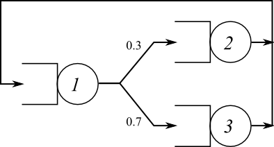
Fig. 1: Three-nodes central server queueing network model (closed network)

The routing probabilities are shown in the picture. To analyze this network we use the qnclosed() function. This function has the following signature:

[U, R, Q, X] = qnclosed (N, S, V, ...)

where N is the number of requests in the (closed) network, S and V are arrays such that S(k) is the service time at center k, and V(k) is the visit count at center k. The visit counts V for a closed network satisfy the equality V*P == V with the additional constraint V(1) == 1. V can be computed from the routing probability matrix P using the qnvisits function, as follows:

P = [0 0.3 0.7; 1 0 0; 1 0 0];
V = qnvisits(P)

V =

   1.00000   0.30000   0.70000

Let us suppose that there are N=10 requests in the system. We let the average service times be S = [1 2 0.8]. We analyze the network as follows:

N = 10;
S = [1 2 0.8];
P = [0 0.3 0.7; 1 0 0; 1 0 0];
V = qnvisits(P);
[U R Q X] = qnclosed( N, S, V )

U =

   0.99139   0.59483   0.55518

R =

   7.4360   4.7531   1.7500

Q =

   7.3719   1.4136   1.2144

X =

   0.99139   0.29742   0.69397

where U is the vector of per-node utilizations, R is the vector of per-node response times, Q is the vector of average queue lenghts and X is the vector of thorughputs. Thus, the utilization of service center 1 is U(1)==0.99139, which is very close to 1.0. We can conclude that the service center 1 is the bottleneck device.

Analyzing open networks is very similar. Consider the open network shown in Fig. 2

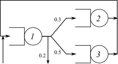
Fig. 2: Three-nodes Central Server Queueing Network Model (Open network)

Assume that the average service times are as in the previous example (S = [1 2 0.8]). Furthermore, assume an external arrival rate of 0.3 requests/s to center 1, and no external arrivals to other centers.

Again, we need first to compute the visit counts. The function qnvisits can be used to compute the visit counts as in the previous example, but in this case we need to pass the vector of external arrival rates as an additional parameter. The vector of external arrival rates is lambda = [0.3 0 0]. Thus, we can issue the following Octave commands:

P = [0 0.3 0.5; 1 0 0; 1 0 0];
lambda = [0.15 0 0];
V = qnvisits(P,lambda)

V =

   5.0000   1.5000   2.5000

We might also verify that the external arrival rate is less than the processing capacity of the network, which by definition is the inverse of the maximum service demand:

S = [1 2 0.8];
D = V .* S

D =

   5.0000   3.0000   2.0000

1/max(D)

ans = 0.20000

sum(lambda)

ans = 0.15000

Since sum(lambda) < 1/max(D), it is possible to analyze the steady-state behavior of the network. We use the qnopen function to compute the results of interest:

[U R Q X] = qnopen( sum(lambda), S, V )

U =

   0.75000   0.45000   0.30000

R =

   4.0000   3.6364   1.1429

Q =

   3.00000   0.81818   0.42857

X =

   0.75000   0.22500   0.37500

Since the queueing network shown in Fig. 2 is a Jackson Network, you can also use the qnjackson function to compute the exact same results using the routing probability matrix P directly.

[U R Q X] = qnjackson(lambda, S, P)

U =

   0.75000   0.45000   0.30000

R =

   4.0000   3.6364   1.1429

Q =

   3.00000   0.81818   0.42857

X =

   0.75000   0.22500   0.37500

Finally, let us see a more complete example. The following is embedded as a demo function of the qnclosed.m source file, and you can execute it by issuing this command at the Octave prompt:

demo("qnclosed.m");

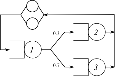
Fig. 3: Three-nodes Central Server Queueing Model (Closed network), with terminals

In this demo we want to compute the bounds on the system throughput for the network in Fig. 3, which is very similar to the one of Fig. 1, with the only addition of an external think time. We are going to use the qnclosedab and qnclosedbsb functions, to compute the bounds on the system throughput for increasing values of the population size N, and compare the results with the exact throughput provided by the MVA algorithm.

P = [0 0.3 0.7; 1 0 0; 1 0 0]; # Transition probability matrix
S = [1 0.6 0.2]; # Average service times
m = ones(1,3);   # All centers are single-server
Z = 2;           # External delay
Nmax = 15;       # Maximum population to consider
V = qnvisits(P); # Compute number of visits from P
D = V .* S;      # Compute service demand from S and V
X_bsb_lower = X_bsb_upper = zeros(1,Nmax);
X_ab_lower = X_ab_upper = zeros(1,Nmax);
X_mva = zeros(1,Nmax);
for n=1:Nmax
  [X_bsb_lower(n) X_bsb_upper(n)] = qnclosedbsb(n, D, Z);
  [X_ab_lower(n) X_ab_upper(n)] = qnclosedab(n, D, Z);
  [U R Q X] = qnclosed( n, S, V, m, Z );
  X_mva(n) = X(1)/V(1);
endfor
close all;
plot(1:Nmax, X_ab_lower,"g;Asymptotic Bounds;", \
     1:Nmax, X_bsb_lower,"k;Balanced System Bounds;", \
     1:Nmax, X_mva,"b;MVA;", "linewidth", 2, \
     1:Nmax, X_bsb_upper,"k", \
     1:Nmax, X_ab_upper,"g" );
title("MVA vs Balanced System Bounds");
axis([1,Nmax,0,1]);
xlabel("Request Population Size N");
ylabel("System Throughput X(N)");
legend("location","southeast");

The result is shown in Fig. 4.

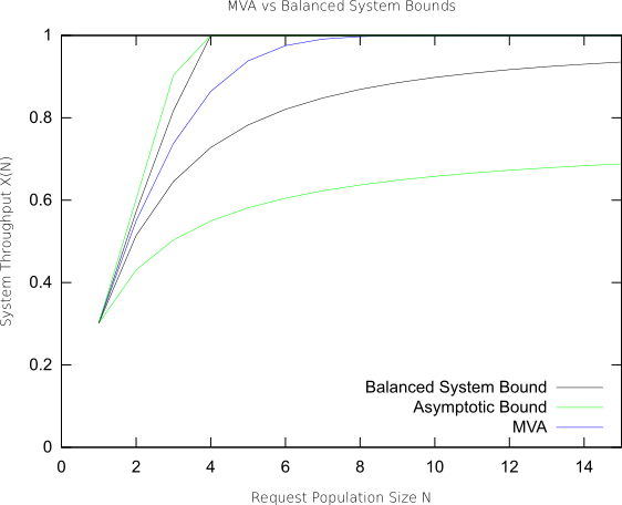
Fig. 4: Balanced Systems Bounds and Asymptotic Bounds on the system throughput X(N) as a function of the population size N for the three-node, closed network in Fig. 3.

Finally, starting from version 0.8.0 of qnetworks, there are a couple of functions which facilitate the definition and analysis of QN models. These functions are qnmknode and qnsolve. The first one is used to create appropriate data structures describing certain kind of QN nodes; the second one is used to analyze a model represented by those data structures. It should be observed that qnsolve (re)implements the same algorithms used by other functions such as qnopensingle, qnclosedsingle and so on; only the input parameters are different.

Consider again the closed network shown in Fig. 3. Using the new functions, the network can be described and analyzed as follows:

P = [0 0.3 0.7; 1 0 0; 1 0 0];
V = qnvisits(P);
QQ = { qnmknode("m/m/m-fcfs", 1), \
       qnmknode("m/m/m-fcfs", 0.6), \
       qnmknode("m/m/m-fcfs", 0.2) };
Z = 2; # external delay
N = 10; # population
[U R Q X] = qnsolve("closed", N, QQ, V, Z); 

The qnmknode function can be used to instantiate different kind of nodes (see the documentation for details). If can also be used to create multi-class nodes, or general load-dependent nodes, which can be analyzed with qnsolve. Again, see the documentation for details.

Return to top

TODO

The software can be improved in many ways:

• Keep the documentation up-to-date; add missing chapters.
• Improve tests coverage.
• Implement additional QN algorithms. Some references are G. Bolch, S. Greiner, H. de Meer, K. Trivedi, Queueing Networks and Markov Chains—Modeling and Performance Evaluation with Computer Science Applications, Wiley, 1998; L. Kleinrock, Queueing Systems Volume 1: Theory, Wiley-Interscience; 1 edition (January 2, 1975), ISBN 978-0471491101.

Return to top

Resources

• Java Modelling Tools (JMT), developed by the Performance Evaluation Lab of the Politecnico di Milano, Italy
• List of Queueing Theory Software, maintained by Myron Hlynka
• Edward D. Lazowska, John Zahorjan, G. Scott Graham, Kenneth C. Sevcik, Quantitative System Performance—Computer System Analysis Using Queueing Network Models, Prentice-Hall, 1984. This book is the source of some of the algorithms implemented in the qnetworks package. Furthermore, the PDF version of the book is freely downloadable.

Return to top

References

- Ian F. Akyildiz, Mean Value Analysis for Blocking Queueing Networks, IEEE Transactions on Software Engineering, vol. 14, n. 2, April 1988, pp. 418—428.
- Y. Bard, Some Extensions to Multiclass Queueing Network Analysis, proc. 4th Int. Symp. on Modelling and Performance Evaluation of Computer Systems, feb. 1979, pp. 51—62
- Forest Baskett, K. Mani Chandy, Richard R. Muntz, and Fernando G. Palacios. 1975. Open, Closed, and Mixed Networks of Queues with Different Classes of Customers. J. ACM 22, 2 (April 1975), 248—260.
- G. Bolch, S. Greiner, H. de Meer and K. Trivedi, Queueing Networks and Markov Chains: Modeling and Performance Evaluation with Computer Science Applications, Wiley, 1998
- Jeffrey P. Buzen, Computational algorithms for closed queueing networks with exponential servers. Commun. ACM 16, 9 (September 1973), 527-531.
- G. Casale, R. R. Muntz, G. Serazzi. Geometric Bounds: a Noniterative Analysis Technique for Closed Queueing Networks, IEEE Transactions on Computers, 57(6):780—794, Jun 2008. doi>
- G. Casale. A Note on Stable Flow-Equivalent Aggregation in Closed Networks, Queueing Systems, 60(3):193-202, Springer, Dec 2008. [SpringerLink]
- C. H. Hsieh and S. Lam, Two classes of performance bounds for closed queueing networks, PEVA, vol. 7, no. 1, pp. 3—30, 1987.
- James R. Jackson, Jobshop-Like Queueing Systems, Vol. 50, No. 12, Ten Most Influential Titles of "Management Science's" First Fifty Years (Dec., 2004), pp. 1796-1802
- Edward D. Lazowska, John Zahorjan, G. Scott Graham, and Kenneth C. Sevcik, Quantitative System Performance: Computer System Analysis Using Queueing Network Models, Prentice Hall, 1984
- M. Reiser and S. S. Lavenberg, Mean-Value Analysis of Closed Multichain Queuing Networks, Journal of the ACM, vol. 27, n. 2, April 1980, pp. 313—322.
- M. Reiser, H. Kobayashi, On The Convolution Algorithm for Separable Queueing Networks, In Proceedings of the 1976 ACM SIGMETRICS Conference on Computer Performance Modeling Measurement and Evaluation (Cambridge, Massachusetts, United States, March 29—31, 1976). SIGMETRICS '76. ACM, New York, NY, pp. 109—117.
- P. Schweitzer, Approximate Analysis of Multiclass Closed Networks of Queues, Proc. Int. Conf. on Stochastic Control and Optimization, jun 1979, pp. 25—29.
- Herb Schwetman, Implementing the Mean Value Algorithm for the Solution of Queueing Network Models, Technical Report CSD-TR-355, Department of Computer Sciences, Purdue University, 1982.
- Herb Schwetman, Some Computational Aspects of Queueing Network Models, Technical Report CSD-TR-354, Department of Computer Sciences, Purdue University, 1981 (revised).
- Zahorjan, J. and Wong, E. The solution of separable queueing network models using mean value analysis. SIGMETRICS Perform. Eval. Rev. 10, 3 (Sep. 1981), 80—85.