queueing

Permission is granted to make and distribute verbatim copies of this manual provided the copyright notice and this permission notice are preserved on all copies.

Permission is granted to copy and distribute modified versions of this manual under the conditions for verbatim copying, provided that the entire resulting derived work is distributed under the terms of a permission notice identical to this one.

Permission is granted to copy and distribute translations of this manual into another language, under the above conditions for modified versions.

1 Summary
2 Installation and Getting Started
3 Markov Chains
- 3.1 Discrete-Time Markov Chains
- 3.2 Continuous-Time Markov Chains
4 Single Station Queueing Systems
5 Queueing Networks
6 References
Appendix A GNU GENERAL PUBLIC LICENSE
Concept Index
Function Index

This manual documents how to install and run the Queueing package. It corresponds to version 1.2.7 of the package.

1 Summary

1.1 About the Queueing Package

This document describes the queueing package for GNU Octave (queueing in short). The queueing package, previously known as qnetworks toolbox, is a collection of functions for analyzing queueing networks and Markov chains written for GNU Octave. Specifically, queueing contains functions for analyzing Jackson networks, open, closed or mixed product-form BCMP networks, and computing performance bounds. The following algorithms are available

Convolution for closed, single-class product-form networks with load-dependent service centers;
Exact and approximate Mean Value Analysis (MVA) for single and multiple class product-form closed networks;
MVA for mixed, multiple class product-form networks with load-independent service centers;
Approximate MVA for closed, single-class networks with blocking (MVABLO algorithm by F. Akyildiz);
Asymptotic Bounds, Balanced System Bounds and Geometric Bounds;

queueing provides functions for analyzing the following types of single-station queueing systems:

M/M/1
M/M/m
M/M/\infty
M/M/1/k single-server, finite capacity system
M/M/m/k multiple-server, finite capacity system
Asymmetric M/M/m
M/G/1 (general service time distribution)
M/H_m/1 (Hyperexponential service time distribution)

Functions for Markov chain analysis are also provided (discrete- and continuous-time chains are supported):

Birth-death processes;
Transient and stationary state occupancy probabilities;
Mean time to absorption;
Expected sojourn times and time-averaged sojourn times;
Mean first passage times;

The queueing package is distributed under the terms of the GNU General Public License (GPL), version 3 or later (see Copying). You are encouraged to share this software with others, and improve this package by contributing additional functions and reporting bugs. See Contributing Guidelines.

If you use the queueing package in a technical paper, please cite it as:

Moreno Marzolla, The qnetworks Toolbox: A Software Package for Queueing Networks Analysis. Khalid Al-Begain, Dieter Fiems and William J. Knottenbelt, Editors, Proceedings 17th International Conference on Analytical and Stochastic Modeling Techniques and Applications (ASMTA 2010) Cardiff, UK, June 14–16, 2010, volume 6148 of Lecture Notes in Computer Science, Springer, pp. 102–116, ISBN 978-3-642-13567-5

If you use BibTeX, this is the citation block:

@inproceedings{queueing,
  author    = {Moreno Marzolla},
  title     = {The qnetworks Toolbox: A Software Package for Queueing 
               Networks Analysis},
  booktitle = {Analytical and Stochastic Modeling Techniques and 
               Applications, 17th International Conference, 
               ASMTA 2010, Cardiff, UK, June 14-16, 2010. Proceedings},
  editor    = {Khalid Al-Begain and Dieter Fiems and William J. Knottenbelt},
  year      = {2010},
  publisher = {Springer},
  series    = {Lecture Notes in Computer Science},
  volume    = {6148},
  pages     = {102--116},
  ee        = {http://dx.doi.org/10.1007/978-3-642-13568-2_8},
  isbn      = {978-3-642-13567-5}
}

An early draft of the paper above is available as Technical Report UBLCS-2010-04, February 2010, Department of Computer Science, University of Bologna, Italy.

1.2 Contributing Guidelines

Contributions and bug reports are always welcome. If you want to contribute to the queueing package, here are some guidelines:

If you are contributing a new function, please embed proper documentation within the function itself. The documentation must be in texinfo format, so that it can be extracted and included into the printable manual. See the existing functions for the documentation style.
Make sure that each new function validates its input parameters. For example, a function accepting vectors should check whether the dimensions match.
Provide bibliographic references for each new algorithm you contribute. Document any significant difference from the reference. Update the doc/references.txi file if appropriate.
Include test and demo blocks. Test blocks are particularly important, since most algorithms are tricky to implement correctly. If appropriate, test blocks should also verify that the function fails on incorrect inputs.

Send your contribution to Moreno Marzolla (moreno.marzolla@unibo.it). If you are a user of this package and find it useful, let me know by dropping me a line. Thanks.

1.3 Acknowledgments

The following people (listed alphabetically) contributed to the queueing package, either by providing feedback, reporting bugs or contributing code: Philip Carinhas, Phil Colbourn, Diego Didona, Yves Durand, Marco Guazzone, Dmitry Kolesnikov, Michele Mazzucco, Marco Paolieri.

2 Installation and Getting Started

2.1 Installation through Octave package management system

The most recent version of queueing is 1.2.7 and can be downloaded from Octave-Forge

https://octave.sourceforge.io/queueing/

Additional information can be found at

http://www.moreno.marzolla.name/software/queueing/

To install queueing, follow these steps:

If you have a recent version of GNU Octave and a network connection, you can install queueing from Octave command prompt using this command:
```
octave:1> pkg install -forge queueing
```
The command above will download and install the latest version of the queueing package from Octave Forge, and install it on your machine.

If you do not have root access, you can perform a local install with:
```
octave:1> pkg install -local -forge queueing
```
This will install queueing in your home directory, and the package will be available to the current user only.
Alternatively, you can first download the queueing tarball from Octave-Forge; to install the package in the system-wide location issue this command at the Octave prompt:
```
octave:1> pkg install queueing-1.2.7.tar.gz
```
(you may need to start Octave as root in order to allow the installation to copy the files to the target locations). After this, all functions will be available each time Octave starts, without the need to tweak the search path.

If you do not have root access, you can do a local install using:
```
octave:1> pkg install -local queueing-1.2.7.tar.gz
```

Use the pkg list command at the Octave prompt to check that the queueing package has been succesfully installed; you should see something like:

octave:1>pkg list queueing
Package Name  | Version | Installation directory
--------------+---------+-----------------------
    queueing  |   1.2.7 | /home/moreno/octave/queueing-1.2.7

Starting from version 1.1.1, queueing is no longer automatically loaded on Octave start. To make the functions available for use, you need to issue the command
```
octave:1>pkg load queueing 
```
at the Octave prompt. To automatically load queueing each time Octave starts, you can add the command above to the startup script (usually, ~/.octaverc on Unix systems).
To completely remove queueing from your system, use the pkg uninstall command:
```
octave:1> pkg uninstall queueing
```

2.2 Manual installation

If you want to manually install queueing in a custom location, you can download the tarball and unpack it somewhere:

tar xvfz queueing-1.2.7.tar.gz
cd queueing-1.2.7/queueing/

Copy all .m files from the inst/ directory to some target location. Then, start Octave with the -p option to add the target location to the search path, so that Octave will find all queueing functions automatically:

octave -p /path/to/queueing

For example, if all queueing m-files are in /usr/local/queueing, you can start Octave as follows:

octave -p /usr/local/queueing

If you want, you can add the following line to ~/.octaverc:

addpath("/path/to/queueing");

so that the path /path/to/queueing is automatically added to the search path each time Octave is started, and you no longer need to specify the -p option on the command line.

2.3 Development sources

The source code of the queueing package can be found in the Mercurial repository at the URL:

https://sourceforge.net/p/octave/queueing/ci/default/tree/

The source distribution contains additional development files that are not present in the installation tarball. This section briefly describes the content of the source tree. This is only relevant for developers who want to modify the code or the documentation.

The source distribution contains the following directories:

doc/: Documentation sources. Most of the documentation is extracted from the comment blocks of function files from the inst/ directory.
inst/: This directory contains the m-files which implement the various algorithms provided by queueing. As a notational convention, the names of functions for Queueing Networks begin with the ‘qn’ prefix; the name of functions for Continuous-Time Markov Chains (CTMCs) begin with the ‘ctmc’ prefix, and the names of functions for Discrete-Time Markov Chains (DTMCs) begin with the ‘dtmc’ prefix.
test/: This directory contains the test scripts used to run all function tests.
devel/: This directory contains functions that are either not working properly, or need additional testing before they are moved to the inst/ directory.

The queueing package ships with a Makefile which can be used to produce the documentation (in PDF and HTML format), and automatically execute all function tests. The following targets are defined:

all: Running ‘make’ (or ‘make all’) on the top-level directory builds the programs used to extract the documentation from the comments embedded in the m-files, and then produce the documentation in PDF and HTML format (doc/queueing.pdf and doc/queueing.html, respectively).
check: Running ‘make check’ will execute all tests contained in the m-files. If you modify the code of any function in the inst/ directory, you should run the tests to ensure that no errors have been introduced. You are also encouraged to contribute new tests, especially for functions that are not adequately validated.
clean
distclean
dist: The ‘make clean’, ‘make distclean’ and ‘make dist’ commands are used to clean up the source directory and prepare the distribution archive in compressed tar format.

2.4 Naming Conventions

Most of the functions in the queueing package obey a common naming convention. Function names are made of several parts; the first part is a prefix which indicates the class of problems the function addresses:

ctmc-: Functions for continuous-time Markov chains
dtmc-: Functions for discrete-time Markov chains
qs-: Functions for analyzing single-station queueing systems (individual service centers)
qn-: Functions for analyzing queueing networks

Functions dealing with Markov chains start with either the ctmc or dtmc prefix; the prefix is optionally followed by an additional string which hints at what the function does:

-bd: Birth-Death process
-mtta: Mean Time to Absorption
-fpt: First Passage Times
-exps: Expected Sojourn Times
-taexps: Time-Averaged Expected Sojourn Times

For example, function ctmcbd returns the infinitesimal generator matrix for a continuous birth-death process, while dtmcbd returns the transition probability matrix for a discrete birth-death process. Note that there exist functions ctmc and dtmc (without any suffix) that compute steady-state and transient state occupancy probabilities for CTMCs and DTMCs, respectively. See Markov Chains.

Functions whose name starts with qs- deal with single station queueing systems. The suffix describes the type of system, e.g., qsmm1 for M/M/1, qnmmm for M/M/m and so on. See Single Station Queueing Systems.

Finally, functions whose name starts with qn- deal with queueing networks. The character that follows indicates whether the function handles open ('o') or closed ('c') networks, and whether there is a single customer class ('s') or multiple classes ('m'). The string mix indicates that the function supports mixed networks with both open and closed customer classes.

-os-: Open, single-class network: open network with a single class of customers
-om-: Open, multiclass network: open network with multiple job classes
-cs-: Closed, single-class network
-cm-: Closed, multiclass network
-mix-: Mixed network with open and closed classes of customers

The last part of the function name indicates the algorithm implemented by the function. See Queueing Networks.

-aba: Asymptotic Bounds Analysis
-bsb: Balanced System Bounds
-gb: Geometric Bounds
-pb: PB Bounds
-cb: Composite Bounds (CB)
-mva: Mean Value Analysis (MVA) algorithm
-cmva: Conditional MVA
-mvald: MVA with general load-dependent servers
-mvaap: Approximate MVA
-mvablo: MVABLO approximation for blocking queueing networks
-conv: Convolution algorithm
-convld: Convolution algorithm with general load-dependent servers

Some deprecated functions may be present in the queueing package; generally, these are functions that have been renamed, and the old name is kept for a while for backward compatibility. Deprecated functions are not documented and will be removed in future releases. Calling a deprecated functions displays a warning message that appears only once per session. The warning message can be turned off with the command:

octave:1> warning ("off", "qn:deprecated-function");

However, you are strongly recommended to update your code to the new API. To help catching usages of deprecated functions, you can transform warnings into errors so that your application stops immediately:

octave:1> warning ("error", "qn:deprecated-function");

2.5 Quick start Guide

You can use all functions by simply invoking their name with the appropriate parameters; an error is shown in case of missing/wrong parameters. Extensive documentation is provided for each function, and can be displayed with the help command. For example:

octave:2> help qncsmvablo

shows the documentation for the qncsmvablo function. Additional information can be found in the queueing manual, that is available in PDF format in doc/queueing.pdf and in HTML format in doc/queueing.html.

Many functions have demo blocks showing usage examples. To execute the demos for the qnclosed function, use the demo command:

octave:4> demo qnclosed

We now illustrate a few examples of how the queueing package can be used. More examples are provided in the manual.

Example 1 Compute the stationary state occupancy probabilities of a continuous-time Markov chain with infinitesimal generator matrix

    / -0.8   0.6   0.2 \
Q = |  0.3  -0.7   0.4 |
    \  0.2   0.2  -0.4 /

Q = [ -0.8  0.6  0.2; \
       0.3 -0.7  0.4; \
       0.2  0.2 -0.4 ];
q = ctmc(Q)
    ⇒ q = 0.23256   0.32558   0.44186

Example 2 Compute the transient state occupancy probability after n=3 transitions of a three state discrete-time birth-death process, with birth probabilities \lambda_{01} = 0.3 and \lambda_{12} = 0.5 and death probabilities \mu_{10} = 0.5 and \mu_{21} = 0.7, assuming that the system is initially in state zero (i.e., the initial state occupancy probabilities are [1, 0, 0]).

n = 3;
p0 = [1 0 0];
P = dtmcbd( [0.3 0.5], [0.5 0.7] );
p = dtmc(P,n,p0)
    ⇒ p = 0.55300   0.29700   0.15000

Example 3 Compute server utilization, response time, mean number of requests and throughput of a closed queueing network with N=4 requests and three M/M/1–FCFS queues with mean service times S = [1.0, 0.8, 1.4] and average number of visits V = [1.0, 0.8, 0.8]

S = [1.0 0.8 1.4];
V = [1.0 0.8 0.8];
N = 4;
[U R Q X] = qncsmva(N, S, V)
    ⇒ 
     U = 0.70064   0.44841   0.78471
     R = 2.1030    1.2642    3.2433
     Q = 1.47346   0.70862   1.81792
     X = 0.70064   0.56051   0.56051

Example 4 Compute server utilization, response time, mean number of requests and throughput of an open queueing network with three M/M/1–FCFS queues with mean service times S = [1.0, 0.8, 1.4] and average number of visits V = [1.0, 0.8, 0.8]. The overall arrival rate is \lambda = 0.8 requests/second.

S = [1.0 0.8 1.4];
V = [1.0 0.8 0.8];
lambda = 0.8;
[U R Q X] = qnos(lambda, S, V)
    ⇒ 
     U = 0.80000   0.51200   0.89600
     R = 5.0000    1.6393   13.4615
     Q = 4.0000    1.0492    8.6154
     X = 0.80000   0.64000   0.64000

3 Markov Chains

3.1 Discrete-Time Markov Chains

Let X_0, X_1, …, X_n, … be a sequence of random variables defined over the discrete state space 1, 2, …. The sequence X_0, X_1, …, X_n, … is a stochastic process with discrete time 0, 1, 2, …. A Markov chain is a stochastic process {X_n, n=0, 1, …} which satisfies the following Markov property:

P(X_{n+1} = x_{n+1} | X_n = x_n, X_{n-1} = x_{n-1}, …, X_0 = x_0) = P(X_{n+1} = x_{n+1} | X_n = x_n)

which basically means that the probability that the system is in a particular state at time n+1 only depends on the state the system was at time n.

The evolution of a Markov chain with finite state space {1, …, N} can be fully described by a stochastic matrix {\bf P}(n) = [ P_{i,j}(n) ] where P_{i, j}(n) = P( X_{n+1} = j\ |\ X_n = i ). If the Markov chain is homogeneous (that is, the transition probability matrix {\bf P}(n) is time-independent), we can write {\bf P} = [P_{i, j}], where P_{i, j} = P( X_{n+1} = j\ |\ X_n = i ) for all n=0, 1, ….

The transition probability matrix \bf P must be a stochastic matrix, meaning that it must satisfy the following two properties:

P_{i, j} ≥ 0 for all 1 ≤ i, j ≤ N;
\sum_{j=1}^N P_{i,j} = 1 for all i

Property 1 requires that all probabilities are nonnegative; property 2 requires that the outgoing transition probabilities from any state i sum to one.

Function File: [r err] = dtmcchkP (P)

Check whether P is a valid transition probability matrix.

If P is valid, r is the size (number of rows or columns) of P. If P is not a transition probability matrix, r is set to zero, and err to an appropriate error string.

A DTMC is irreducible if every state can be reached with non-zero probability starting from every other state.

Function File: [r s] = dtmcisir (P)

Check if P is irreducible, and identify Strongly Connected Components (SCC) in the transition graph of the DTMC with transition matrix P.

INPUTS

P(i,j): transition probability from state i to state j. P must be an N \times N stochastic matrix.

OUTPUTS

r: 1 if P is irreducible, 0 otherwise (scalar)
s(i): strongly connected component (SCC) that state i belongs to (vector of length N). SCCs are numbered 1, 2, …. The number of SCCs is max(s). If the graph is strongly connected, then there is a single SCC and the predicate all(s == 1) evaluates to true

3.1.1 State occupancy probabilities

Given a discrete-time Markov chain with state space {1, …, N}, we denote with {\bf \pi}(n) = \left[\pi_1(n), … \pi_N(n) \right] the state occupancy probability vector at step n = 0, 1, …. \pi_i(n) is the probability that the system is in state i after n transitions.

Given the transition probability matrix \bf P and the initial state occupancy probability vector {\bf \pi}(0) = \left[\pi_1(0), …, \pi_N(0)\right], {\bf \pi}(n) can be computed as:

\pi(n) = \pi(0) P^n

Under certain conditions, there exists a stationary state occupancy probability {\bf \pi} = \lim_{n \rightarrow +\infty} {\bf \pi}(n), which is independent from {\bf \pi}(0). The vector \bf \pi is the solution of the following linear system:

/
| \pi P   = \pi
| \pi 1^T = 1
\

where \bf 1 is the row vector of ones, and ( \cdot )^T the transpose operator.

Function File: p = dtmc (P)

Function File: p = dtmc (P, n, p0)

Compute stationary or transient state occupancy probabilities for a discrete-time Markov chain.

With a single argument, compute the stationary state occupancy probabilities p(1), …, p(N) for a discrete-time Markov chain with finite state space {1, …, N} and with N \times N transition matrix P. With three arguments, compute the transient state occupancy probabilities p(1), …, p(N) that the system is in state i after n steps, given initial occupancy probabilities p0(1), …, p0(N).

INPUTS

P(i,j): transition probabilities from state i to state j. P must be an N \times N irreducible stochastic matrix, meaning that the sum of each row must be 1 (\sum_{j=1}^N P_{i, j} = 1), and the rank of P must be N.
n: Number of transitions after which state occupancy probabilities are computed (scalar, n ≥ 0)
p0(i): probability that at step 0 the system is in state i (vector of length N).

OUTPUTS

p(i): If this function is called with a single argument, p(i) is the steady-state probability that the system is in state i. If this function is called with three arguments, p(i) is the probability that the system is in state i after n transitions, given the probabilities p0(i) that the initial state is i.

See also: ctmc.

EXAMPLE

The following example is from GrSn97. Let us consider a maze with nine rooms, as shown in the following figure

+-----+-----+-----+
|     |     |     |
|  1     2     3  |
|     |     |     |
+-   -+-   -+-   -+
|     |     |     |
|  4     5     6  |
|     |     |     |
+-   -+-   -+-   -+
|     |     |     |
|  7     8     9  |
|     |     |     |
+-----+-----+-----+

A mouse is placed in one of the rooms and can wander around. At each step, the mouse moves from the current room to a neighboring one with equal probability. For example, if it is in room 1, it can move to room 2 and 4 with probability 1/2, respectively; if the mouse is in room 8, it can move to either 7, 5 or 9 with probability 1/3.

The transition probabilities P_{i, j} from room i to room j can be summarized in the following matrix:

        / 0     1/2   0     1/2   0     0     0     0     0   \
        | 1/3   0     1/3   0     1/3   0     0     0     0   |
        | 0     1/2   0     0     0     1/2   0     0     0   |
        | 1/3   0     0     0     1/3   0     1/3   0     0   |
    P = | 0     1/4   0     1/4   0     1/4   0     1/4   0   |
        | 0     0     1/3   0     1/3   0     0     0     1/3 |
        | 0     0     0     1/2   0     0     0     1/2   0   |
        | 0     0     0     0     1/3   0     1/3   0     1/3 |
        \ 0     0     0     0     0     1/2   0     1/2   0   /

The stationary state occupancy probabilities can then be computed with the following code:

 P = zeros(9,9);
 P(1,[2 4]    ) = 1/2;
 P(2,[1 5 3]  ) = 1/3;
 P(3,[2 6]    ) = 1/2;
 P(4,[1 5 7]  ) = 1/3;
 P(5,[2 4 6 8]) = 1/4;
 P(6,[3 5 9]  ) = 1/3;
 P(7,[4 8]    ) = 1/2;
 P(8,[7 5 9]  ) = 1/3;
 P(9,[6 8]    ) = 1/2;
 p = dtmc(P);
 disp(p)

    ⇒ 0.083333   0.125000   0.083333   0.125000   
       0.166667   0.125000   0.083333   0.125000   
       0.083333

3.1.2 Birth-death process

Function File: P = dtmcbd (b, d)

Returns the transition probability matrix P for a discrete birth-death process over state space {1, …, N}. For each i=1, …, (N-1), b(i) is the transition probability from state i to (i+1), and d(i) is the transition probability from state (i+1) to i.

Matrix \bf P is defined as:

/                                                             \
| 1-b(1)     b(1)                                             |
|  d(1)  (1-d(1)-b(2))     b(2)                               |
|            d(2)      (1-d(2)-b(3))     b(3)                 |
|                                                             |
|                 ...           ...          ...              |
|                                                             |
|                         d(N-2)   (1-d(N-2)-b(N-1))  b(N-1)  |
|                                        d(N-1)      1-d(N-1) |
\                                                             /

where \lambda_i and \mu_i are the birth and death probabilities, respectively.

See also: ctmcbd.

3.1.3 Expected Number of Visits

Given a N state discrete-time Markov chain with transition matrix \bf P and an integer n ≥ 0, we let L_i(n) be the the expected number of visits to state i during the first n transitions. The vector {\bf L}(n) = \left[ L_1(n), …, L_N(n) \right] is defined as

         n            n
        ___          ___
       \            \           i
L(n) =  >   pi(i) =  >   pi(0) P
       /___         /___
        i=0          i=0

where {\bf \pi}(i) = {\bf \pi}(0){\bf P}^i is the state occupancy probability after i transitions, and {\bf \pi}(0) = \left[\pi_1(0), …, \pi_N(0) \right] are the initial state occupancy probabilities.

If \bf P is absorbing, i.e., the stochastic process eventually enters a state with no outgoing transitions, then we can compute the expected number of visits until absorption \bf L. To do so, we first rearrange the states by rewriting \bf P as

    / Q | R \
P = |---+---|
    \ 0 | I /

where the first t states are transient and the last r states are absorbing (t+r = N). The matrix {\bf N} = ({\bf I} - {\bf Q})^{-1} is called the fundamental matrix; N_{i,j} is the expected number of times the process is in the j-th transient state assuming it started in the i-th transient state. If we reshape \bf N to the size of \bf P (filling missing entries with zeros), we have that, for absorbing chains, {\bf L} = {\bf \pi}(0){\bf N}.

Function File: L = dtmcexps (P, n, p0)

Function File: L = dtmcexps (P, p0)

Compute the expected number of visits to each state during the first n transitions, or until abrosption.

INPUTS

P(i,j): N \times N transition matrix. P(i,j) is the transition probability from state i to state j.
n: Number of steps during which the expected number of visits are computed (n ≥ 0). If n=0, returns p0. If n > 0, returns the expected number of visits after exactly n transitions.
p0(i): Initial state occupancy probabilities; p0(i) is the probability that the system is in state i at step 0.

OUTPUTS

L(i): When called with two arguments, L(i) is the expected number of visits to state i before absorption. When called with three arguments, L(i) is the expected number of visits to state i during the first n transitions.

REFERENCES

Grinstead, Charles M.; Snell, J. Laurie (July 1997). Introduction to Probability, Ch. 11: Markov Chains. American Mathematical Society. ISBN 978-0821807491.

See also: ctmcexps.

3.1.4 Time-averaged expected sojourn times

Function File: M = dtmctaexps (P, n, p0)

Function File: M = dtmctaexps (P, p0)

Compute the time-averaged sojourn times M(i), defined as the fraction of time spent in state i during the first n transitions (or until absorption), assuming that the state occupancy probabilities at time 0 are p0.

INPUTS

P(i,j): N \times N transition probability matrix.
n: Number of transitions during which the time-averaged expected sojourn times are computed (scalar, n ≥ 0). if n = 0, returns p0.
p0(i): Initial state occupancy probabilities (vector of length N).

OUTPUTS

M(i): If this function is called with three arguments, M(i) is the expected fraction of steps {0, …, n} spent in state i, assuming that the state occupancy probabilities at time zero are p0. If this function is called with two arguments, M(i) is the expected fraction of steps spent in state i until absorption. M is a vector of length N.

See also: dtmcexps.

3.1.5 Mean Time to Absorption

The mean time to absorption is defined as the average number of transitions that are required to enter an absorbing state, starting from a transient state or given initial state occupancy probabilities {\bf \pi}(0).

Let t_i be the expected number of transitions before being absorbed in any absorbing state, starting from state i. The vector {\bf t} = [t_1, …, t_N] can be computed from the fundamental matrix \bf N (see Expected number of visits (DTMC)) as

t = N c

where \bf c is a column vector of 1’s.

Let {\bf B} = [ B_{i, j} ] be a matrix where B_{i, j} is the probability of being absorbed in state j, starting from transient state i. Again, using matrices \bf N and \bf R (see Expected number of visits (DTMC)) we can write

B = N R

Function File: [t N B] = dtmcmtta (P)

Function File: [t N B] = dtmcmtta (P, p0)

Compute the expected number of steps before absorption for a DTMC with state space {1, …, N} and transition probability matrix P.

INPUTS

P(i,j): N \times N transition probability matrix. P(i,j) is the transition probability from state i to state j.
p0(i): Initial state occupancy probabilities (vector of length N).

OUTPUTS

t
t(i): When called with a single argument, t is a vector of length N such that t(i) is the expected number of steps before being absorbed in any absorbing state, starting from state i; if i is absorbing, t(i) = 0. When called with two arguments, t is a scalar, and represents the expected number of steps before absorption, starting from the initial state occupancy probability p0.
N(i)
N(i,j): When called with a single argument, N is the N \times N fundamental matrix for P. N(i,j) is the expected number of visits to transient state j before absorption, if the system started in transient state i. The initial state is counted if i = j. When called with two arguments, N is a vector of length N such that N(j) is the expected number of visits to transient state j before absorption, given initial state occupancy probability P0.
B(i)
B(i,j): When called with a single argument, B is a N \times N matrix where B(i,j) is the probability of being absorbed in state j, starting from transient state i; if j is not absorbing, B(i,j) = 0; if i is absorbing, B(i,i) = 1 and B(i,j) = 0 for all i \neq j. When called with two arguments, B is a vector of length N where B(j) is the probability of being absorbed in state j, given initial state occupancy probabilities p0.

REFERENCES

Grinstead, Charles M.; Snell, J. Laurie (July 1997). Introduction to Probability, Ch. 11: Markov Chains. American Mathematical Society. ISBN 978-0821807491.

See also: ctmcmtta.

3.1.6 First Passage Times

The First Passage Time M_{i, j} is the average number of transitions needed to enter state j for the first time, starting from state i. Matrix \bf M satisfies the property

           ___
          \
M_ij = 1 + >   P_ij * M_kj
          /___
          k!=j

To compute {\bf M} = [ M_{i, j}] a different formulation is used. Let \bf W be the N \times N matrix having each row equal to the stationary state occupancy probability vector \bf \pi for \bf P; let \bf I be the N \times N identity matrix (i.e., the matrix of all ones). Define \bf Z as follows:

               -1
Z = (I - P + W)

Then, we have that

       Z_jj - Z_ij
M_ij = -----------
          \pi_j

According to the definition above, M_{i,i} = 0. We arbitrarily set M_{i,i} to the mean recurrence time r_i for state i, that is the average number of transitions needed to return to state i starting from it. r_i is:

        1
r_i = -----
      \pi_i

Function File: M = dtmcfpt (P)

Compute mean first passage times and mean recurrence times for an irreducible discrete-time Markov chain over the state space {1, …, N}.

INPUTS

P(i,j): transition probability from state i to state j. P must be an irreducible stochastic matrix, which means that the sum of each row must be 1 (\sum_{j=1}^N P_{i j} = 1), and the rank of P must be N.

OUTPUTS

M(i,j): For all 1 ≤ i, j ≤ N, i \neq j, M(i,j) is the average number of transitions before state j is entered for the first time, starting from state i. M(i,i) is the mean recurrence time of state i, and represents the average time needed to return to state i.

REFERENCES

Grinstead, Charles M.; Snell, J. Laurie (July 1997). Introduction to Probability, Ch. 11: Markov Chains. American Mathematical Society. ISBN 978-0821807491.

See also: ctmcfpt.

3.2 Continuous-Time Markov Chains

A stochastic process {X(t), t ≥ 0} is a continuous-time Markov chain if, for all integers n, and for any sequence t_0, t_1 , …, t_n, t_{n+1} such that t_0 < t_1 < … < t_n < t_{n+1}, we have

P(X_{n+1} = x_{n+1} | X_n = x_n, X_{n-1} = x_{n-1}, ..., X_0 = x_0) = P(X_{n+1} = x_{n+1} | X_n = x_n)

A continuous-time Markov chain is defined according to an infinitesimal generator matrix {\bf Q} = [Q_{i,j}], where for each i \neq j, Q_{i, j} is the transition rate from state i to state j. The matrix \bf Q must satisfy the property that, for all i, \sum_{j=1}^N Q_{i, j} = 0.

Function File: [result err] = ctmcchkQ (Q): If Q is a valid infinitesimal generator matrix, return the size (number of rows or columns) of Q. If Q is not an infinitesimal generator matrix, set result to zero, and err to an appropriate error string.

Similarly to the DTMC case, a CTMC is irreducible if every state is eventually reachable from every other state in finite time.

Function File: [r s] = ctmcisir (P)

Check if Q is irreducible, and identify Strongly Connected Components (SCC) in the transition graph of the DTMC with infinitesimal generator matrix Q.

INPUTS

Q(i,j): Infinitesimal generator matrix. Q is a N \times N square matrix where Q(i,j) is the transition rate from state i to state j, for 1 ≤ i, j ≤ N, i \neq j.

OUTPUTS

r: 1 if Q is irreducible, 0 otherwise.
s(i): strongly connected component (SCC) that state i belongs to. SCCs are numbered 1, 2, …. If the graph is strongly connected, then there is a single SCC and the predicate all(s == 1) evaluates to true.

3.2.1 State occupancy probabilities

Similarly to the discrete case, we denote with {\bf \pi}(t) = \left[\pi_1(t), …, \pi_N(t) \right] the state occupancy probability vector at time t. \pi_i(t) is the probability that the system is in state i at time t ≥ 0.

Given the infinitesimal generator matrix \bf Q and initial state occupancy probabilities {\bf \pi}(0) = \left[\pi_1(0), …, \pi_N(0)\right], the occupancy probabilities {\bf \pi}(t) at time t can be computed as:

\pi(t) = \pi(0) exp(Qt)

where \exp( {\bf Q} t ) is the matrix exponential of {\bf Q} t. Under certain conditions, there exists a stationary state occupancy probability {\bf \pi} = \lim_{t \rightarrow +\infty} {\bf \pi}(t) that is independent from {\bf \pi}(0). \bf \pi is the solution of the following linear system:

/
| \pi Q   = 0
| \pi 1^T = 1
\

Function File: p = ctmc (Q)

Function File: p = ctmc (Q, t, p0)

Compute stationary or transient state occupancy probabilities for a continuous-time Markov chain.

With a single argument, compute the stationary state occupancy probabilities p(1), …, p(N) for a continuous-time Markov chain with finite state space {1, …, N} and N \times N infinitesimal generator matrix Q. With three arguments, compute the state occupancy probabilities p(1), …, p(N) that the system is in state i at time t, given initial state occupancy probabilities p0(1), …, p0(N) at time 0.

INPUTS

Q(i,j): Infinitesimal generator matrix. Q is a N \times N square matrix where Q(i,j) is the transition rate from state i to state j, for 1 ≤ i \neq j ≤ N. Q must satisfy the property that \sum_{j=1}^N Q_{i, j} = 0
t: Time at which to compute the transient probability (t ≥ 0). If omitted, the function computes the steady state occupancy probability vector.
p0(i): probability that the system is in state i at time 0.

OUTPUTS

p(i): If this function is invoked with a single argument, p(i) is the steady-state probability that the system is in state i, i = 1, …, N. If this function is invoked with three arguments, p(i) is the probability that the system is in state i at time t, given the initial occupancy probabilities p0(1), …, p0(N).

See also: dtmc.

EXAMPLE

Consider a two-state CTMC where all transition rates between states are equal to 1. The stationary state occupancy probabilities can be computed as follows:

 Q = [ -1  1; ...
        1 -1  ];
 q = ctmc(Q)

    ⇒ q = 0.50000   0.50000

3.2.2 Birth-Death Process

Function File: Q = ctmcbd (b, d)

Returns the infinitesimal generator matrix Q for a continuous birth-death process over the finite state space {1, …, N}. For each i=1, …, (N-1), b(i) is the transition rate from state i to state (i+1), and d(i) is the transition rate from state (i+1) to state i.

Matrix \bf Q is therefore defined as:

/                                                          \
| -b(1)     b(1)                                           |
|  d(1) -(d(1)+b(2))     b(2)                              |
|           d(2)     -(d(2)+b(3))        b(3)              |
|                                                          |
|                ...           ...          ...            |
|                                                          |
|                       d(N-2)    -(d(N-2)+b(N-1))  b(N-1) |
|                                       d(N-1)     -d(N-1) |
\                                                          /

where \lambda_i and \mu_i are the birth and death rates, respectively.

See also: dtmcbd.

3.2.3 Expected Sojourn Times

Given a N state continuous-time Markov Chain with infinitesimal generator matrix \bf Q, we define the vector {\bf L}(t) = \left[L_1(t), …, L_N(t)\right] such that L_i(t) is the expected sojourn time in state i during the interval [0,t), assuming that the initial occupancy probabilities at time 0 were {\bf \pi}(0). {\bf L}(t) can be expressed as the solution of the following differential equation:

 dL
 --(t) = L(t) Q + pi(0),    L(0) = 0
 dt

Alternatively, {\bf L}(t) can also be expressed in integral form as:

       / t
L(t) = |   pi(u) du
       / 0

where {\bf \pi}(t) = {\bf \pi}(0) \exp({\bf Q}t) is the state occupancy probability at time t; \exp({\bf Q}t) is the matrix exponential of {\bf Q}t.

If there are absorbing states, we can define the vector of expected sojourn times until absorption {\bf L}(\infty), where for each transient state i, L_i(\infty) is the expected total time spent in state i until absorption, assuming that the system started with given state occupancy probabilities {\bf \pi}(0). Let \tau be the set of transient (i.e., non absorbing) states; let {\bf Q}_\tau be the restriction of \bf Q to the transient sub-states only. Similarly, let {\bf \pi}_\tau(0) be the restriction of the initial state occupancy probability vector {\bf \pi}(0) to transient states \tau.

The expected time to absorption {\bf L}_\tau(\infty) is defined as the solution of the following equation:

L_T( inf ) Q_T = -pi_T(0)

Function File: L = ctmcexps (Q, t, p )

Function File: L = ctmcexps (Q, p)

With three arguments, compute the expected times L(i) spent in each state i during the time interval [0,t], assuming that the initial occupancy vector is p. With two arguments, compute the expected time L(i) spent in each transient state i until absorption.

Note: In its current implementation, this function requires that an absorbing state is reachable from any non-absorbing state of Q.

INPUTS

Q(i,j): N \times N infinitesimal generator matrix. Q(i,j) is the transition rate from state i to state j, 1 ≤ i, j ≤ N, i \neq j. The matrix Q must also satisfy the condition \sum_{j=1}^N Q_{i,j} = 0 for every i=1, …, N.
t: If given, compute the expected sojourn times in [0,t]
p(i): Initial occupancy probability vector; p(i) is the probability the system is in state i at time 0, i = 1, …, N

OUTPUTS

L(i): If this function is called with three arguments, L(i) is the expected time spent in state i during the interval [0,t]. If this function is called with two arguments L(i) is the expected time spent in transient state i until absorption; if state i is absorbing, L(i) is zero.

See also: dtmcexps.

EXAMPLE

Let us consider a 4-states pure birth continuous process where the transition rate from state i to state (i+1) is \lambda_i = i \lambda (i=1, 2, 3), with \lambda = 0.5. The following code computes the expected sojourn time for each state i, given initial occupancy probabilities {\bf \pi}_0=[1, 0, 0, 0].

 lambda = 0.5;
 N = 4;
 b = lambda*[1:N-1];
 d = zeros(size(b));
 Q = ctmcbd(b,d);
 t = linspace(0,10,100);
 p0 = zeros(1,N); p0(1)=1;
 L = zeros(length(t),N);
 for i=1:length(t)
   L(i,:) = ctmcexps(Q,t(i),p0);
 endfor
 plot( t, L(:,1), ";State 1;", "linewidth", 2, ...
       t, L(:,2), ";State 2;", "linewidth", 2, ...
       t, L(:,3), ";State 3;", "linewidth", 2, ...
       t, L(:,4), ";State 4;", "linewidth", 2 );
 legend("location","northwest"); legend("boxoff");
 xlabel("Time");
 ylabel("Expected sojourn time");

3.2.4 Time-Averaged Expected Sojourn Times

Function File: M = ctmctaexps (Q, t, p0)

Function File: M = ctmctaexps (Q, p0)

Compute the time-averaged sojourn time M(i), defined as the fraction of the time interval [0,t] (or until absorption) spent in state i, assuming that the state occupancy probabilities at time 0 are p.

INPUTS

Q(i,j): Infinitesimal generator matrix. Q(i,j) is the transition rate from state i to state j, 1 ≤ i,j ≤ N, i \neq j. The matrix Q must also satisfy the condition \sum_{j=1}^N Q_{i,j} = 0
t: Time. If omitted, the results are computed until absorption.
p0(i): initial state occupancy probabilities. p0(i) is the probability that the system is in state i at time 0, i = 1, …, N

OUTPUTS

M(i): When called with three arguments, M(i) is the expected fraction of the interval [0,t] spent in state i assuming that the state occupancy probability at time zero is p. When called with two arguments, M(i) is the expected fraction of time until absorption spent in state i; in this case the mean time to absorption is sum(M).

See also: ctmcexps.

EXAMPLE

 lambda = 0.5;
 N = 4;
 birth = lambda*linspace(1,N-1,N-1);
 death = zeros(1,N-1);
 Q = diag(birth,1)+diag(death,-1);
 Q -= diag(sum(Q,2));
 t = linspace(1e-5,30,100);
 p = zeros(1,N); p(1)=1;
 M = zeros(length(t),N);
 for i=1:length(t)
   M(i,:) = ctmctaexps(Q,t(i),p);
 endfor
 clf;
 plot(t, M(:,1), ";State 1;", "linewidth", 2, ...
      t, M(:,2), ";State 2;", "linewidth", 2, ...
      t, M(:,3), ";State 3;", "linewidth", 2, ...
      t, M(:,4), ";State 4 (absorbing);", "linewidth", 2 );
 legend("location","east"); legend("boxoff");
 xlabel("Time");
 ylabel("Time-averaged Expected sojourn time");

3.2.5 Mean Time to Absorption

Function File: t = ctmcmtta (Q, p)

Compute the Mean-Time to Absorption (MTTA) of the CTMC described by the infinitesimal generator matrix Q, starting from initial occupancy probabilities p. If there are no absorbing states, this function fails with an error.

INPUTS

Q(i,j): N \times N infinitesimal generator matrix. Q(i,j) is the transition rate from state i to state j, i \neq j. The matrix Q must satisfy the condition \sum_{j=1}^N Q_{i,j} = 0
p(i): probability that the system is in state i at time 0, for each i=1, …, N

OUTPUTS

t: Mean time to absorption of the process represented by matrix Q. If there are no absorbing states, this function fails.

REFERENCES

G. Bolch, S. Greiner, H. de Meer and K. Trivedi, Queueing Networks and Markov Chains: Modeling and Performance Evaluation with Computer Science Applications, Wiley, 1998.

See also: ctmcexps.

EXAMPLE

Let us consider a simple model of redundant disk array. We assume that the array is made of 5 independent disks and can tolerate up to 2 disk failures without losing data. If three or more disks break, the array is dead and unrecoverable. We want to estimate the Mean-Time-To-Failure (MTTF) of the disk array.

We model this system as a 4 states continuous Markov chain with state space { 2, 3, 4, 5 }. In state i there are exactly i active (i.e., non failed) disks; state 2 is absorbing. Let \mu be the failure rate of a single disk. The system starts in state 5 (all disks are operational). We use a pure death process, where the death rate from state i to state (i-1) is \mu i, for i = 3, 4, 5).

The MTTF of the disk array is the MTTA of the Markov Chain, and can be computed as follows:

 mu = 0.01;
 death = [ 3 4 5 ] * mu;
 birth = 0*death;
 Q = ctmcbd(birth,death);
 t = ctmcmtta(Q,[0 0 0 1])

    ⇒ t = 78.333

3.2.6 First Passage Times

Function File: M = ctmcfpt (Q)

Function File: m = ctmcfpt (Q, i, j)

Compute mean first passage times for an irreducible continuous-time Markov chain.

INPUTS

Q(i,j): Infinitesimal generator matrix. Q is a N \times N square matrix where Q(i,j) is the transition rate from state i to state j, for 1 ≤ i, j ≤ N, i \neq j. Transition rates must be nonnegative, and \sum_{j=1}^N Q_{i,j} = 0
i: Initial state.
j: Destination state.

OUTPUTS

M(i,j): average time before state j is visited for the first time, starting from state i. We let M(i,i) = 0.
m: m is the average time before state j is visited for the first time, starting from state i.

See also: ctmcmtta.

4 Single Station Queueing Systems

Single Station Queueing Systems contain a single station, and can usually be analyzed easily. The queueing package contains functions for handling the following types of queues:

• The M/M/1 System:		Single-server queueing station.
• The M/M/m System:		Multiple-server queueing station.
• The Erlang-B Formula:
• The Erlang-C Formula:
• The Engset Formula:
• The M/M/inf System:		Infinite-server (delay center) station.
• The M/M/1/K System:		Single-server, finite-capacity queueing station.
• The M/M/m/K System:		Multiple-server, finite-capacity queueing station.
• The Asymmetric M/M/m System:		Asymmetric multiple-server queueing station.
• The M/G/1 System:		Single-server with general service time distribution.
• The M/Hm/1 System:		Single-server with hyperexponential service time distribution.

4.1 The M/M/1 System

The M/M/1 system contains a single server connected to an unbounded FCFS queue. Requests arrive according to a Poisson process with rate \lambda; the service time is exponentially distributed with average service rate \mu. The system is stable if \lambda < \mu.

Function File: [U, R, Q, X, p0] = qsmm1 (lambda, mu)

Function File: pk = qsmm1 (lambda, mu, k)

Compute utilization, response time, average number of requests and throughput for a M/M/1 queue.

INPUTS

lambda: Arrival rate (lambda ≥ 0).
mu: Service rate (mu > lambda).
k: Number of requests in the system (k ≥ 0).

OUTPUTS

U: Server utilization
R: Server response time
Q: Average number of requests in the system
X: Server throughput. If the system is ergodic (mu > lambda), we always have X = lambda
p0: Steady-state probability that there are no requests in the system.
pk: Steady-state probability that there are k requests in the system. (including the one being served).

If this function is called with less than three input parameters, lambda and mu can be vectors of the same size. In this case, the results will be vectors as well.

REFERENCES

G. Bolch, S. Greiner, H. de Meer and K. Trivedi, Queueing Networks and Markov Chains: Modeling and Performance Evaluation with Computer Science Applications, Wiley, 1998, Section 6.3

See also: qsmmm, qsmminf, qsmmmk.

4.2 The M/M/m System

The M/M/m system is similar to the M/M/1 system, except that there are m \geq 1 identical servers connected to a shared FCFS queue. Thus, at most m requests can be served at the same time. The M/M/m system can be seen as a single server with load-dependent service rate \mu(n), which is a function of the number n of requests in the system:

mu(n) = min(m,n)*mu

where \mu is the service rate of each individual server.

Function File: [U, R, Q, X, p0, pm] = qsmmm (lambda, mu)

Function File: [U, R, Q, X, p0, pm] = qsmmm (lambda, mu, m)

Function File: pk = qsmmm (lambda, mu, m, k)

Compute utilization, response time, average number of requests in service and throughput for a M/M/m queue, a queueing system with m identical servers connected to a single FCFS queue.

INPUTS

lambda: Arrival rate (lambda>0).
mu: Service rate (mu>lambda).
m: Number of servers (m ≥ 1). Default is m=1.
k: Number of requests in the system (k ≥ 0).

OUTPUTS

U: Service center utilization, U = \lambda / (m \mu).
R: Service center mean response time
Q: Average number of requests in the system
X: Service center throughput. If the system is ergodic, we will always have X = lambda
p0: Steady-state probability that there are 0 requests in the system
pm: Steady-state probability that an arriving request has to wait in the queue
pk: Steady-state probability that there are k requests in the system (including the one being served).

If this function is called with less than four parameters, lambda, mu and m can be vectors of the same size. In this case, the results will be vectors as well.

REFERENCES

G. Bolch, S. Greiner, H. de Meer and K. Trivedi, Queueing Networks and Markov Chains: Modeling and Performance Evaluation with Computer Science Applications, Wiley, 1998, Section 6.5

See also: erlangc,qsmm1,qsmminf,qsmmmk.

4.3 The Erlang-B Formula

Function File: B = erlangb (A, m)

Compute the steady-state blocking probability in the Erlang loss model.

The Erlang-B formula E_B(A, m) gives the probability that an open system with m identical servers, arrival rate \lambda, individual service rate \mu and offered load A = \lambda / \mu has all servers busy. This corresponds to the rejection probability of an M/M/m/0 system with m servers and no queue.

INPUTS

A: Offered load, defined as A = \lambda / \mu where \lambda is the mean arrival rate and \mu the mean service rate of each individual server (real, A > 0).
m: Number of identical servers (integer, m ≥ 1). Default m = 1

OUTPUTS

B: The value E_B(A, m)

A or m can be vectors, and in this case, the results will be vectors as well.

REFERENCES

G. Zeng, Two common properties of the Erlang-B function, Erlang-C function, and Engset blocking function, Mathematical and Computer Modelling, Volume 37, Issues 12-13, June 2003, Pages 1287-1296

See also: erlangc,engset,qsmmm.

4.4 The Erlang-C Formula

Function File: C = erlangc (A, m)

Compute the steady-state probability of delay in the Erlang delay model.

The Erlang-C formula E_C(A, m) gives the probability that an open queueing system with m identical servers, infinite wating space, arrival rate \lambda, individual service rate \mu and offered load A = \lambda / \mu has all the servers busy. This is the waiting probability in an M/M/m/\infty system with m servers and an infinite queue.

INPUTS

A: Offered load. A = \lambda / \mu where \lambda is the mean arrival rate and \mu the mean service rate of each individual server (real, 0 < A < m).
m: Number of identical servers (integer, m ≥ 1). Default m = 1

OUTPUTS

B: The value E_C(A, m)

A or m can be vectors, and in this case, the results will be vectors as well.

REFERENCES

G. Zeng, Two common properties of the Erlang-B function, Erlang-C function, and Engset blocking function, Mathematical and Computer Modelling, Volume 37, Issues 12-13, June 2003, Pages 1287-1296

See also: erlangb,engset,qsmmm.

4.5 The Engset Formula

Function File: B = engset (A, m, n)

Evaluate the Engset loss formula.

The Engset formula computes the blocking probability P_b(A,m,n) for a system with a finite population of n users, m identical servers, no queue, individual service rate \mu, individual arrival rate \lambda (i.e., the time until a user tries to request service is exponentially distributed with mean 1/\lambda), and offered load A=\lambda/\mu.

INPUTS

A: Offered load, defined as A = \lambda / \mu where \lambda is the mean arrival rate and \mu the mean service rate of each individual server (real, A > 0).
m: Number of identical servers (integer, m ≥ 1). Default m = 1
n: Number of requests (integer, n ≥ 1). Default n = 1

OUTPUTS

B: The value P_b(A, m, n)

A, m or n can be vectors, and in this case, the results will be vectors as well.

REFERENCES

G. Zeng, Two common properties of the Erlang-B function, Erlang-C function, and Engset blocking function, Mathematical and Computer Modelling, Volume 37, Issues 12-13, June 2003, Pages 1287-1296

See also: erlangb, erlangc.

4.6 The M/M/inf System

The M/M/\infty system is a special case of M/M/m system with infinitely many identical servers (i.e., m = \infty). Each new request is always assigned to a new server, so that queueing never occurs. The M/M/\infty system is always stable.

Function File: [U, R, Q, X, p0] = qsmminf (lambda, mu)

Function File: pk = qsmminf (lambda, mu, k)

Compute utilization, response time, average number of requests and throughput for an infinite-server queue.

The M/M/\infty system has an infinite number of identical servers. Such a system is always stable (i.e., the mean queue length is always finite) for any arrival and service rates.

INPUTS

lambda: Arrival rate (lambda>0).
mu: Service rate (mu>0).
k: Number of requests in the system (k ≥ 0).

OUTPUTS

U: Traffic intensity (defined as \lambda/\mu). Note that this is different from the utilization, which in the case of M/M/\infty centers is always zero.
R: Service center response time.
Q: Average number of requests in the system (which is equal to the traffic intensity \lambda/\mu).
X: Throughput (which is always equal to X = lambda).
p0: Steady-state probability that there are no requests in the system
pk: Steady-state probability that there are k requests in the system (including the one being served).

If this function is called with less than three arguments, lambda and mu can be vectors of the same size. In this case, the results will be vectors as well.

REFERENCES

G. Bolch, S. Greiner, H. de Meer and K. Trivedi, Queueing Networks and Markov Chains: Modeling and Performance Evaluation with Computer Science Applications, Wiley, 1998, Section 6.4

See also: qsmm1,qsmmm,qsmmmk.

4.7 The M/M/1/K System

In a M/M/1/K finite capacity system there is a single server, and there can be at most K jobs at any time (including the job currently in service), K > 1. If a new request tries to join the system when there are already K other requests, the request is lost. The queue has K-1 slots. The M/M/1/K system is always stable, regardless of the arrival and service rates.

Function File: [U, R, Q, X, p0, pK] = qsmm1k (lambda, mu, K)

Function File: pn = qsmm1k (lambda, mu, K, n)

Compute utilization, response time, average number of requests and throughput for a M/M/1/K finite capacity system.

In a M/M/1/K queue there is a single server and a queue with finite capacity: the maximum number of requests in the system (including the request being served) is K, and the maximum queue length is therefore K-1.

INPUTS

lambda: Arrival rate (lambda>0).
mu: Service rate (mu>0).
K: Maximum number of requests allowed in the system (K ≥ 1).
n: Number of requests in the (0 ≤ n ≤ K).

OUTPUTS

U: Service center utilization, which is defined as U = 1-p0
R: Service center response time
Q: Average number of requests in the system
X: Service center throughput
p0: Steady-state probability that there are no requests in the system
pK: Steady-state probability that there are K requests in the system (i.e., that the system is full)
pn: Steady-state probability that there are n requests in the system (including the one being served).

If this function is called with less than four arguments, lambda, mu and K can be vectors of the same size. In this case, the results will be vectors as well.

See also: qsmm1,qsmminf,qsmmm.

4.8 The M/M/m/K System

The M/M/m/K finite capacity system is similar to the M/M/1/k system except that the number of servers is m, where 1 \leq m \leq K. The queue has K-m slots. The M/M/m/K system is always stable.

Function File: [U, R, Q, X, p0, pK] = qsmmmk (lambda, mu, m, K)

Function File: pn = qsmmmk (lambda, mu, m, K, n)

Compute utilization, response time, average number of requests and throughput for a M/M/m/K finite capacity system. In a M/M/m/K system there are m \geq 1 identical service centers sharing a fixed-capacity queue. At any time, at most K ≥ m requests can be in the system, including those being served. The maximum queue length is K-m. This function generates and solves the underlying CTMC.

INPUTS

lambda: Arrival rate (lambda>0)
mu: Service rate (mu>0)
m: Number of servers (m ≥ 1)
K: Maximum number of requests allowed in the system, including those being served (K ≥ m)
n: Number of requests in the (0 ≤ n ≤ K).

OUTPUTS

U: Service center utilization
R: Service center response time
Q: Average number of requests in the system
X: Service center throughput
p0: Steady-state probability that there are no requests in the system.
pK: Steady-state probability that there are K requests in the system (i.e., probability that the system is full).
pn: Steady-state probability that there are n requests in the system (including those being served).

If this function is called with less than five arguments, lambda, mu, m and K can be either scalars, or vectors of the same size. In this case, the results will be vectors as well.

REFERENCES

G. Bolch, S. Greiner, H. de Meer and K. Trivedi, Queueing Networks and Markov Chains: Modeling and Performance Evaluation with Computer Science Applications, Wiley, 1998, Section 6.6

See also: qsmm1,qsmminf,qsmmm.

4.9 The Asymmetric M/M/m System

The Asymmetric M/M/m system contains m servers connected to a single queue. Differently from the M/M/m system, in the asymmetric M/M/m each server may have a different service time.

Function File: [U, R, Q, X] = qsammm (lambda, mu)

Compute approximate utilization, response time, average number of requests in service and throughput for an asymmetric M/M/m queue. In this type of system there are m different servers connected to a single queue. Each server has its own (possibly different) service rate. If there is more than one server available, requests are routed to a randomly-chosen one.

INPUTS

lambda: Arrival rate (lambda>0)
mu: mu(i) is the service rate of server i, 1 ≤ i ≤ m. The system must be ergodic (lambda < sum(mu)).

OUTPUTS

U: Approximate service center utilization, U = \lambda / ( \sum_{i=1}^m \mu_i ).
R: Approximate service center response time
Q: Approximate number of requests in the system
X: Approximate system throughput. If the system is ergodic, X = lambda

REFERENCES

G. Bolch, S. Greiner, H. de Meer and K. Trivedi, Queueing Networks and Markov Chains: Modeling and Performance Evaluation with Computer Science Applications, Wiley, 1998

See also: qsmmm.

4.10 The M/G/1 System

Function File: [U, R, Q, X, p0] = qsmg1 (lambda, xavg, x2nd)

Compute utilization, response time, average number of requests and throughput for a M/G/1 system. The service time distribution is described by its mean xavg, and by its second moment x2nd. The computations are based on results from L. Kleinrock, Queuing Systems, Wiley, Vol 2, and Pollaczek-Khinchine formula.

INPUTS

lambda: Arrival rate
xavg: Average service time
x2nd: Second moment of service time distribution

OUTPUTS

U: Service center utilization
R: Service center response time
Q: Average number of requests in the system
X: Service center throughput
p0: Probability that there is not any request at system

lambda, xavg, t2nd can be vectors of the same size. In this case, the results will be vectors as well.

See also: qsmh1.

4.11 The M/H_m/1 System

Function File: [U, R, Q, X, p0] = qsmh1 (lambda, mu, alpha)

Compute utilization, response time, average number of requests and throughput for a M/H_m/1 system. In this system, the customer service times have hyper-exponential distribution:

       ___ m
       \
B(x) =  >  alpha(j) * (1-exp(-mu(j)*x))   x>0
       /__ 
           j=1

where \alpha_j is the probability that the request is served at phase j, in which case the average service rate is \mu_j. After completing service at phase j, for some j, the request exits the system.

INPUTS

lambda: Arrival rate
mu: mu(j) is the phase j service rate. The total number of phases m is length(mu).
alpha: alpha(j) is the probability that a request is served at phase j. alpha must have the same size as mu.

OUTPUTS

U: Service center utilization
R: Service center response time
Q: Average number of requests in the system
X: Service center throughput

5 Queueing Networks

5.1 Introduction to QNs

Queueing Networks (QN) are a simple modeling notation that can be used to analyze many kinds of systems. In its simplest form, a QN is made of K service centers; center k has a queue connected to m_k (usually identical) servers. Arriving customers (requests) join the queue if there is at least one slot available. Requests are served according to a (de)queueing policy (e.g., FIFO). After service completes, requests leave the server and can join another queue or exit from the system.

Service centers where m_k = \infty are called delay centers or infinite servers. In this kind of centers, there is always one available server, so that queueing never occurs.

Requests join the queue according to a queueing policy, such as:

FCFS: First-Come-First-Served
LCFS-PR: Last-Come-First-Served, Preemptive Resume
PS: Processor Sharing
IS: Infinite Server (m_k = \infty).

Queueing networks can be open or closed. In open networks there is an infinite population of requests; new customers are generated outside the system, and eventually leave the network. In closed networks there is a fixed population of request that never leave the system.

Queueing models can have a single request class (single class models), meaning that all requests behave in the same way (e.g., they spend the same average time on each particular server). In multiple class models there are multiple request classes, each with its own parameters (e.g., with different service times or different routing probabilities). Furthermore, in multiclass models there can be open and closed chains of requests at the same time.

A particular class of QN models, product-form networks, is of particular interest. Product-form networks fulfill the following assumptions:

The network can consist of open and closed job classes.
The following queueing disciplines are allowed: FCFS, PS, LCFS-PR and IS.
Service times for FCFS nodes must be exponentially distributed and class-independent. Service centers at PS, LCFS-PR and IS nodes can have any kind of service time distribution with a rational Laplace transform. Furthermore, for PS, LCFS-PR and IS nodes, different classes of customers can have different service times.
The service rate of an FCFS node is only allowed to depend on the number of jobs at this node; in a PS, LCFS-PR and IS node the service rate for a particular job class can also depend on the number of jobs of that class at the node.
In open networks two kinds of arrival processes are allowed: i) the arrival process is Poisson, with arrival rate \lambda that can depend on the number of jobs in the network. ii) the arrival process consists of C independent Poisson arrival streams where the C job sources are assigned to the C chains; the arrival rate can be load dependent.

Product-form networks are attractive because steady-state performance measures can be efficiently computed.

5.2 Single Class Models

In single class models, all requests are indistinguishable and belong to the same class. This means that every request has the same average service time, and all requests move through the system with the same routing probabilities.

Model Inputs

{lambda}_k: (Open models only) External arrival rate to service center k.
lambda: (Open models only) Overall external arrival rate to the system as a whole: \lambda = \sum_k \lambda_k.
N: (Closed models only) Total number of requests in the system.
S_k: Mean service time at center k. S_k is the average time elapsed from service start to service completion at center k.
P_{i, j}: Routing probability matrix. {\bf P} = [P_{i, j}] is a K \times K matrix where P_{i, j} is the probability that a request completing service at center i is routed to center j. The probability that a request leaves the system after being served at center i is \left(1-\sum_{j=1}^K P_{i, j}\right).
V_k: Mean number of visits to center k (also called visit ratio or relative arrival rate).

Model Outputs

U_k: Utilization of service center k. The utilization is defined as the fraction of time in which the resource is busy (i.e., the server is processing requests). If center k is a single-server or multiserver node, then 0 ≤ U_k ≤ 1. If center k is an infinite server node (delay center), then U_k denotes the traffic intensity and is defined as U_k = X_k S_k; in this case the utilization may be greater than one.
R_k: Average response time of service center k, defined as the mean time between the arrival of a request in the queue and service completion of the same request.
Q_k: Average number of requests in center k; this includes both the requests in the queue and those being served.
X_k: Throughput of service center k. The throughput is the rate of job completions, i.e., the average number of jobs completed over a given time interval.

Given the output parameters above, additional performance measures can be computed:

X: System throughput, X = X_k / V_k for any k for which V_k \neq 0
R: System response time, R = \sum_{k=1}^K R_k V_k
Q: Average number of requests in the system, Q = \sum_{k=1}^K Q_k; for closed systems, this can be written as Q = N-XZ;

For open, single class models, the scalar \lambda denotes the external arrival rate of requests to the system. The average number of visits V_j satisfy the following equation:

                  K
                 ___
                \
V_j = P_(0, j) + >   V_i P_(i, j)    j=1,...,K
                /___
                 i=1

where P_{0, j} is the probability that an external request goes to center j. If we denote with \lambda_j the external arrival rate to center j, and \lambda = \sum_j \lambda_j the overall external arrival rate, then P_{0, j} = \lambda_j / \lambda.

For closed models, the visit ratios satisfy the following equation:

/
|         K
|        ___
|       \
| V_j =  >   V_i P_(i, j)     j=1,...,K
|       /___
|        i=1
|
| V_r = 1                     for a selected reference station r
\

Note that the set of traffic equations V_j = \sum_{i=1}^K V_i P_{i, j} alone can only be solved up to a multiplicative constant; to get a unique solution we impose an additional constraint V_r = 1 for some 1 ≤ r ≤ K. This constraint is equivalent to defining station r as the reference station; the default is r=1, see doc-qncsvisits. A job that returns to the reference station is assumed to have completed its activity cycle. The network throughput is set to the throughput of the reference station.

Function File: V = qncsvisits (P)

Function File: V = qncsvisits (P, r)

Compute the mean number of visits to the service centers of a single class, closed network with K service centers.

INPUTS

P(i,j): probability that a request which completed service at center i is routed to center j (K \times K matrix). For closed networks it must hold that sum(P,2)==1. The routing graph must be strongly connected, meaning that each node must be reachable from every other node.
r: Index of the reference station, r \in {1, …, K}; Default r=1. The traffic equations are solved by imposing the condition V(r) = 1. A request returning to the reference station completes its activity cycle.

OUTPUTS

V(k): average number of visits to service center k, assuming r as the reference station.

Function File: V = qnosvisits (P, lambda)

Compute the average number of visits to the service centers of a single class open Queueing Network with K service centers.

INPUTS

P(i,j): is the probability that a request which completed service at center i is routed to center j (K \times K matrix).
lambda(k): external arrival rate to center k.

OUTPUTS

V(k): average number of visits to server k.

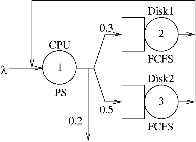
EXAMPLE

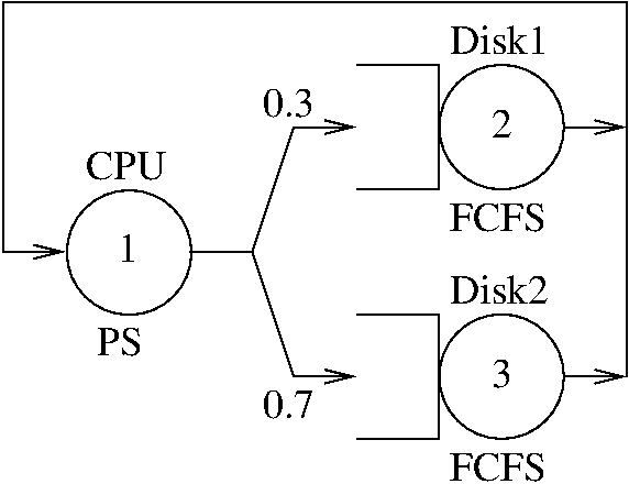
Figure 5.1: Closed network with a single class of requests

Figure 5.1 shows a closed queueing network with a single class of requests. The network has three service centers, labeled CPU, Disk1 and Disk2, and is known as a central server model of a computer system. Requests spend some time at the CPU, which is represented by a PS (Processor Sharing) node. After that, requests are routed to Disk1 with probability 0.3, and to Disk2 with probability 0.7. Both Disk1 and Disk2 are FCFS nodes.

If we label the servers as CPU=1, Disk1=2, Disk2=3, we can define the routing matrix as follows:

    / 0  0.3  0.7 \
P = | 1  0    0   |
    \ 1  0    0   /

The visit ratios V, using station 1 as the reference station, can be computed with:

 P = [0 0.3 0.7; ...
      1 0   0  ; ...
      1 0   0  ];
 V = qncsvisits(P)

   ⇒ V = 1.00000   0.30000   0.70000

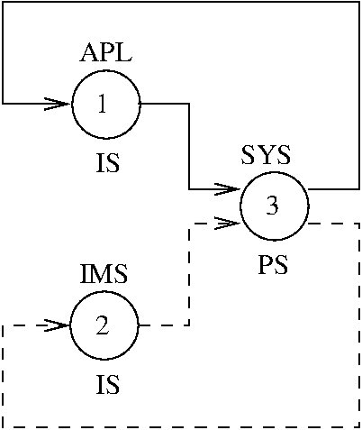
EXAMPLE

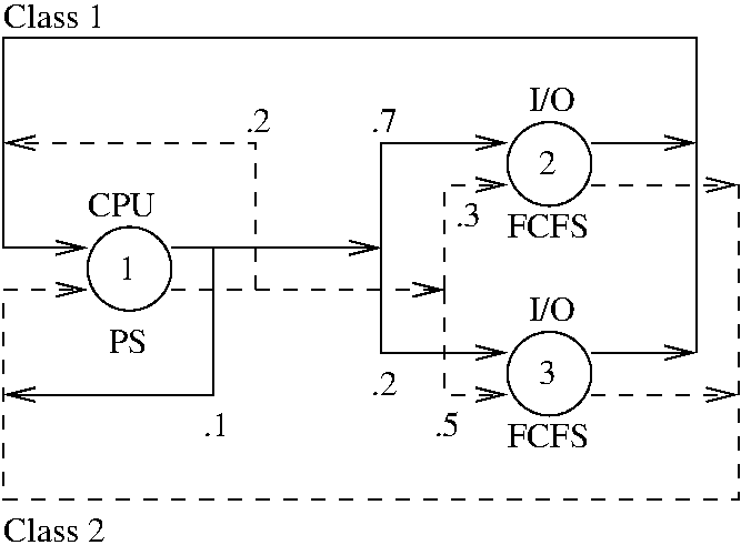
Figure 5.2: Open Queueing Network with a single class of requests

Figure 5.2 shows a open QN with a single class of requests. The network has the same structure as the one in Figure 5.1, with the difference that here we have a stream of jobs arriving from outside the system, at a rate \lambda. After service completion at the CPU, a job can leave the system with probability 0.2, or be transferred to other nodes with the probabilities shown in the figure.

The routing matrix is

    / 0  0.3  0.5 \
P = | 1  0    0   |
    \ 1  0    0   /

If we let \lambda = 1.2, we can compute the visit ratios V as follows:

 p = 0.3;
 lambda = 1.2
 P = [0 0.3 0.5; ...
      1 0   0  ; ...
      1 0   0  ];
 V = qnosvisits(P,[1.2 0 0])

   ⇒ V = 5.0000   1.5000   2.5000

Function qnosvisits expects a vector with K elements as a second parameter, for open networks only. The vector contains the arrival rates at each individual node; since in our example external arrivals exist only for node S_1 with rate \lambda = 1.2, the second parameter is [1.2, 0, 0].

5.2.1 Open Networks

Jackson networks satisfy the following conditions:

There is only one job class in the network; the total number of jobs in the system is unbounded.
There are K service centers in the network. Each service center may have Poisson arrivals from outside the system. A job can leave the system from any node.
Arrival rates as well as routing probabilities are independent from the number of nodes in the network.
External arrivals and service times at the service centers are exponentially distributed, and in general can be load-dependent.
Service discipline at each node is FCFS

We define the joint probability vector \pi(n_1, …, n_K) as the steady-state probability that there are n_k requests at service center k, for all k=1, …, N. Jackson networks have the property that the joint probability is the product of the marginal probabilities \pi_k:

joint_prob = prod( pi )

where \pi_k(n_k) is the steady-state probability that there are n_k requests at service center k.

Function File: [U, R, Q, X] = qnos (lambda, S, V)

Function File: [U, R, Q, X] = qnos (lambda, S, V, m)

Analyze open, single class BCMP queueing networks with K service centers.

This function works for a subset of BCMP single-class open networks satisfying the following properties:

The allowed service disciplines at network nodes are: FCFS, PS, LCFS-PR, IS (infinite server);
Service times are exponentially distributed and load-independent;
Center k can consist of m(k) ≥ 1 identical servers.
Routing is load-independent

INPUTS

lambda: Overall external arrival rate (lambda>0).
S(k): average service time at center k (S(k)>0).
V(k): average number of visits to center k (V(k) ≥ 0).
m(k): number of servers at center i. If m(k) < 1, enter k is a delay center (IS); otherwise it is a regular queueing center with m(k) servers. Default is m(k) = 1 for all k.

OUTPUTS

U(k): If k is a queueing center, U(k) is the utilization of center k. If k is an IS node, then U(k) is the traffic intensity defined as X(k)*S(k).
R(k): center k average response time.
Q(k): average number of requests at center k.
X(k): center k throughput.

REFERENCES

G. Bolch, S. Greiner, H. de Meer and K. Trivedi, Queueing Networks and Markov Chains: Modeling and Performance Evaluation with Computer Science Applications, Wiley, 1998

See also: qnopen,qnclosed,qnosvisits.

From the results computed by this function, it is possible to derive other quantities of interest as follows:

System Response Time: The overall system response time can be computed as R_s = dot(V,R);
Average number of requests: The average number of requests in the system can be computed as: Q_avg = sum(Q)

EXAMPLE

 lambda = 3;
 V = [16 7 8];
 S = [0.01 0.02 0.03];
 [U R Q X] = qnos( lambda, S, V );
 R_s = dot(R,V) # System response time
 N = sum(Q) # Average number in system

-| R_s =  1.4062
-| N =  4.2186

5.2.2 Closed Networks

Function File: [U, R, Q, X, G] = qncsmva (N, S, V)

Function File: [U, R, Q, X, G] = qncsmva (N, S, V, m)

Function File: [U, R, Q, X, G] = qncsmva (N, S, V, m, Z)

Analyze closed, single class queueing networks using the exact Mean Value Analysis (MVA) algorithm.

The following queueing disciplines are supported: FCFS, LCFS-PR, PS and IS (Infinite Server). This function supports fixed-rate service centers or multiple server nodes. For general load-dependent service centers, use the function qncsmvald instead.

Additionally, the normalization constant G(n), n=0, …, N is computed; G(n) can be used in conjunction with the BCMP theorem to compute steady-state probabilities.

INPUTS

N: Population size (number of requests in the system, N ≥ 0). If N == 0, this function returns U = R = Q = X = 0
S(k): mean service time at center k (S(k) ≥ 0).
V(k): average number of visits to service center k (V(k) ≥ 0).
Z: External delay for customers (Z ≥ 0). Default is 0.
m(k): number of servers at center k (if m is a scalar, all centers have that number of servers). If m(k) < 1, center k is a delay center (IS); otherwise it is a regular queueing center (FCFS, LCFS-PR or PS) with m(k) servers. Default is m(k) = 1 for all k (each service center has a single server).

OUTPUTS

U(k): If k is a FCFS, LCFS-PR or PS node (m(k) ≥ 1), then U(k) is the utilization of center k, 0 ≤ U(k) ≤ 1. If k is an IS node (m(k) < 1), then U(k) is the traffic intensity defined as X(k)*S(k). In this case the value of U(k) may be greater than one.
R(k): center k response time. The Residence Time at center k is R(k) * V(k). The system response time Rsys can be computed either as Rsys = N/Xsys - Z or as Rsys = dot(R,V)
Q(k): average number of requests at center k. The number of requests in the system can be computed either as sum(Q), or using the formula N-Xsys*Z.
X(k): center K throughput. The system throughput Xsys can be computed as Xsys = X(1) / V(1)
G(n): Normalization constants. G(n+1) contains the value of the normalization constant G(n), n=0, …, N as array indexes in Octave start from 1. G(n) can be used in conjunction with the BCMP theorem to compute steady-state probabilities.

NOTES

In presence of load-dependent servers (i.e., if m(k)>1 for some k), the MVA algorithm is known to be numerically unstable. Generally, this issue manifests itself as negative values for the response times or utilizations. This is not a problem of the queueing toolbox, but of the MVA algorithm, and has currently no known solution. This function prints a warning if numerical problems are detected; the warning can be disabled with the command warning("off", "qn:numerical-instability").

REFERENCES

M. Reiser and S. S. Lavenberg, Mean-Value Analysis of Closed Multichain Queuing Networks, Journal of the ACM, vol. 27, n. 2, April 1980, pp. 313–322. 10.1145/322186.322195

This implementation is described in R. Jain , The Art of Computer Systems Performance Analysis, Wiley, 1991, p. 577. Multi-server nodes are treated according to G. Bolch, S. Greiner, H. de Meer and K. Trivedi, Queueing Networks and Markov Chains: Modeling and Performance Evaluation with Computer Science Applications, Wiley, 1998, Section 8.2.1, "Single Class Queueing Networks".

See also: qncsmvald,qncscmva.

EXAMPLE

 S = [ 0.125 0.3 0.2 ];
 V = [ 16 10 5 ];
 N = 20;
 m = ones(1,3);
 Z = 4;
 [U R Q X] = qncsmva(N,S,V,m,Z);
 X_s = X(1)/V(1); # System throughput
 R_s = dot(R,V); # System response time
 printf("\t    Util      Qlen     RespT      Tput\n");
 printf("\t--------  --------  --------  --------\n");
 for k=1:length(S)
   printf("Dev%d\t%8.4f  %8.4f  %8.4f  %8.4f\n", k, U(k), Q(k), R(k), X(k) );
 endfor
 printf("\nSystem\t          %8.4f  %8.4f  %8.4f\n\n", N-X_s*Z, R_s, X_s );

Function File: [U, R, Q, X] = qncsmvald (N, S, V)

Function File: [U, R, Q, X] = qncsmvald (N, S, V, Z)

Mean Value Analysis algorithm for closed, single class queueing networks with K service centers and load-dependent service times. This function supports FCFS, LCFS-PR, PS and IS nodes. For networks with only fixed-rate centers and multiple-server nodes, the function qncsmva is more efficient.

INPUTS

N: Population size (number of requests in the system, N ≥ 0). If N == 0, this function returns U = R = Q = X = 0
S(k,n): mean service time at center k where there are n requests, 1 ≤ n ≤ N. S(k,n) = 1 / \mu_{k}(n), where \mu_{k}(n) is the service rate of center k when there are n requests.
V(k): average number of visits to service center k (V(k) ≥ 0).
Z: external delay ("think time", Z ≥ 0); default 0.

OUTPUTS

U(k): utilization of service center k. The utilization is defined as the probability that service center k is not empty, that is, U_k = 1-\pi_k(0) where \pi_k(0) is the steady-state probability that there are 0 jobs at service center k.
R(k): response time on service center k.
Q(k): average number of requests in service center k.
X(k): throughput of service center k.

NOTES

In presence of load-dependent servers, the MVA algorithm is known to be numerically unstable. Generally this problem manifests itself as negative response times or utilization.

REFERENCES

M. Reiser and S. S. Lavenberg, Mean-Value Analysis of Closed Multichain Queuing Networks, Journal of the ACM, vol. 27, n. 2, April 1980, pp. 313–322. 10.1145/322186.322195

This implementation is described in G. Bolch, S. Greiner, H. de Meer and K. Trivedi, Queueing Networks and Markov Chains: Modeling and Performance Evaluation with Computer Science Applications, Wiley, 1998, Section 8.2.4.1, “Networks with Load-Dependent Service: Closed Networks”.

See also: qncsmva.

Function File: [U, R, Q, X] = qncscmva (N, S, Sld, V)

Function File: [U, R, Q, X] = qncscmva (N, S, Sld, V, Z)

Conditional MVA (CMVA) algorithm, a numerically stable variant of MVA. This function supports a network of M ≥ 1 service centers and a single delay center. Servers 1, …, (M-1) are load-independent; server M is load-dependent.

INPUTS

N: Number of requests in the system, N ≥ 0. If N == 0, this function returns U = R = Q = X = 0
S(k): mean service time on server k = 1, …, (M-1) (S(k) > 0). If there are no fixed-rate servers, then S = []
Sld(n): inverse service rate at server M (the load-dependent server) when there are n requests, n=1, …, N. Sld(n) = 1 / \mu(n).
V(k): average number of visits to service center k=1, …, M, where V(k) ≥ 0. V(1:M-1) are the visit rates to the fixed rate servers; V(M) is the visit rate to the load dependent server.
Z: External delay for customers (Z ≥ 0). Default is 0.

OUTPUTS

U(k): center k utilization (k=1, …, M)
R(k): response time of center k (k=1, …, M). The system response time Rsys can be computed as Rsys = N/Xsys - Z
Q(k): average number of requests at center k (k=1, …, M).
X(k): center k throughput (k=1, …, M).

REFERENCES

G. Casale. A note on stable flow-equivalent aggregation in closed networks. Queueing Syst. Theory Appl., 60:193â-202, December 2008, 10.1007/s11134-008-9093-6

Function File: [U, R, Q, X] = qncsmvaap (N, S, V)

Function File: [U, R, Q, X] = qncsmvaap (N, S, V, m)

Function File: [U, R, Q, X] = qncsmvaap (N, S, V, m, Z)

Function File: [U, R, Q, X] = qncsmvaap (N, S, V, m, Z, tol)

Function File: [U, R, Q, X] = qncsmvaap (N, S, V, m, Z, tol, iter_max)

Analyze closed, single class queueing networks using the Approximate Mean Value Analysis (MVA) algorithm. This function is based on approximating the number of customers seen at center k when a new request arrives as Q_k(N) \times (N-1)/N. This function only handles single-server and delay centers; if your network contains general load-dependent service centers, use the function qncsmvald instead.

INPUTS

N: Population size (number of requests in the system, N > 0).
S(k): mean service time on server k (S(k)>0).
V(k): average number of visits to service center k (V(k) ≥ 0).
m(k): number of servers at center k (if m is a scalar, all centers have that number of servers). If m(k) < 1, center k is a delay center (IS); if m(k) == 1, center k is a regular queueing center (FCFS, LCFS-PR or PS) with one server (default). This function does not support multiple server nodes (m(k) > 1).
Z: External delay for customers (Z ≥ 0). Default is 0.
tol: Stopping tolerance. The algorithm stops when the maximum relative difference between the new and old value of the queue lengths Q becomes less than the tolerance. Default is 10^{-5}.
iter_max: Maximum number of iterations (iter_max>0. The function aborts if convergenge is not reached within the maximum number of iterations. Default is 100.

OUTPUTS

U(k): If k is a FCFS, LCFS-PR or PS node (m(k) == 1), then U(k) is the utilization of center k. If k is an IS node (m(k) < 1), then U(k) is the traffic intensity defined as X(k)*S(k).
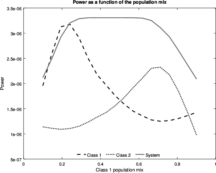
R(k): response time at center k. The system response time Rsys can be computed as Rsys = N/Xsys - Z
Q(k): average number of requests at center k. The number of requests in the system can be computed either as sum(Q), or using the formula N-Xsys*Z.
X(k): center k throughput. The system throughput Xsys can be computed as Xsys = X(1) / V(1)

REFERENCES

See also: qncsmva,qncsmvald.

According to the BCMP theorem, the state probability of a closed single class queueing network with K nodes and N requests can be expressed as:

n = [n1, … nK]; population vector
p = 1/G(N+1) \prod F(k,k);

Here \pi(n_1, …, n_K) is the joint probability of having n_k requests at node k, for all k=1, …, K; we have that \sum_{k=1}^K n_k = N

The convolution algorithms computes the normalization constants {\bf G} = \left[G(0), …, G(N)\right] for single-class, closed networks with N requests. The normalization constants are returned as vector G=[G(1), … G(N+1)] where G(i+1) is the value of G(i) (remember that Octave uses 1-base vectors). The normalization constant can be used to compute all performance measures of interest (utilization, average response time and so on).

queueing implements the convolution algorithm, in the function qncsconv and qncsconvld. The first one supports single-station nodes, multiple-station nodes and IS nodes. The second one supports networks with general load-dependent service centers.

Function File: [U, R, Q, X, G] = qncsconv (N, S, V)

Function File: [U, R, Q, X, G] = qncsconv (N, S, V, m)

Analyze product-form, single class closed networks with K service centers using the convolution algorithm.

Load-independent service centers, multiple servers (M/M/m queues) and IS nodes are supported. For general load-dependent service centers, use qncsconvld instead.

INPUTS

N: Number of requests in the system (N>0).
S(k): average service time on center k (S(k) ≥ 0).
V(k): visit count of service center k (V(k) ≥ 0).
m(k): number of servers at center k. If m(k) < 1, center k is a delay center (IS); if m(k) ≥ 1, center k it is a regular M/M/m queueing center with m(k) identical servers. Default is m(k) = 1 for all k.

OUTPUT

U(k): center k utilization. For IS nodes, U(k) is the traffic intensity X(k) * S(k).
R(k): average response time of center k.
Q(k): average number of customers at center k.
X(k): throughput of center k.
G(n): Vector of normalization constants. G(n+1) contains the value of the normalization constant with n requests G(n), n=0, …, N.

NOTE

For a network with K service centers and N requests, this implementation of the convolution algorithm has time and space complexity O(NK).

REFERENCES

Jeffrey P. Buzen, Computational Algorithms for Closed Queueing Networks with Exponential Servers, Communications of the ACM, volume 16, number 9, September 1973, pp. 527–531. 10.1145/362342.362345

See also: qncsconvld.

EXAMPLE

The normalization constant G can be used to compute the steady-state probabilities for a closed single class product-form Queueing Network with K nodes and N requests. Let n = [n_1, …, n_K] be a valid population vector, \sum_{k=1}^K n_k = N. Then, the steady-state probability p(k) to have n(k) requests at service center k can be computed as:

 n = [1 2 0];
 N = sum(n); # Total population size
 S = [ 1/0.8 1/0.6 1/0.4 ];
 m = [ 2 3 1 ];
 V = [ 1 .667 .2 ];
 [U R Q X G] = qncsconv( N, S, V, m );
 p = [0 0 0]; # initialize p
 # Compute the probability to have n(k) jobs at service center k
 for k=1:3
   p(k) = (V(k)*S(k))^n(k) / G(N+1) * ...
          (G(N-n(k)+1) - V(k)*S(k)*G(N-n(k)) );
   printf("Prob( n(%d) = %d )=%f\n", k, n(k), p(k) );
 endfor

-| Prob( n(1) = 1 ) = 0.17975
-| Prob( n(2) = 2 ) = 0.48404
-| Prob( n(3) = 0 ) = 0.52779

(recall that G(N+1) represents G(N), since in Octave array indices start at one).

Function File: [U, R, Q, X, G] = qncsconvld (N, S, V)

Convolution algorithm for product-form, single-class closed queueing networks with K general load-dependent service centers.

This function computes steady-state performance measures for single-class, closed networks with load-dependent service centers using the convolution algorithm; the normalization constants are also computed. The normalization constants are returned as vector G=[G(1), …, G(N+1)] where G(i+1) is the value of G(i).

INPUTS

N: Number of requests in the system (N>0).
S(k,n): mean service time at center k where there are n requests, 1 ≤ n ≤ N. S(k,n) = 1 / \mu_{k,n}, where \mu_{k,n} is the service rate of center k when there are n requests.
V(k): visit count of service center k (V(k) ≥ 0). The length of V is the number of servers K in the network.

OUTPUT

U(k): center k utilization.
R(k): average response time at center k.
Q(k): average number of requests in center k.
X(k): center k throughput.
G(n): Normalization constants (vector). G(n+1) corresponds to G(n), as array indexes in Octave start from 1.

REFERENCES

Herb Schwetman, Some Computational Aspects of Queueing Network Models, Technical Report CSD-TR-354, Department of Computer Sciences, Purdue University, February 1981 (revised).
M. Reiser, H. Kobayashi, On The Convolution Algorithm for Separable Queueing Networks, In Proceedings of the 1976 ACM SIGMETRICS Conference on Computer Performance Modeling Measurement and Evaluation (Cambridge, Massachusetts, United States, March 29–31, 1976). SIGMETRICS ’76. ACM, New York, NY, pp. 109–117. 10.1145/800200.806187

This implementation is based on G. Bolch, S. Greiner, H. de Meer and K. Trivedi, Queueing Networks and Markov Chains: Modeling and Performance Evaluation with Computer Science Applications, Wiley, 1998, pp. 313–317. Function qncsconvld is slightly different from the version described in Bolch et al. because it supports general load-dependent centers (while the version in the book does not). The modification is in the definition of function F() in qncsconvld which has been made similar to function f_i defined in Schwetman, Some Computational Aspects of Queueing Network Models.

See also: qncsconv.

5.2.3 Non Product-Form QNs

Function File: [U, R, Q, X] = qncsmvablo (N, S, M, P )

Approximate MVA algorithm for closed queueing networks with blocking.

INPUTS

N: number of requests in the system. N must be strictly greater than zero, and less than the overall network capacity: 0 < N < sum(M).
S(k): average service time on server k (S(k) > 0).
M(k): capacity of center k. The capacity is the maximum number of requests in a service center, including the request in service (M(k) ≥ 1).
P(i,j): probability that a request which completes service at server i will be transferred to server j.

OUTPUTS

U(k): center k utilization.
R(k): average response time of service center k.
Q(k): average number of requests in service center k (including the request in service).
X(k): center k throughput.

REFERENCES

Ian F. Akyildiz, Mean Value Analysis for Blocking Queueing Networks, IEEE Transactions on Software Engineering, vol. 14, n. 2, april 1988, pp. 418–428. 10.1109/32.4663

See also: qnopen, qnclosed.

Function File: [U, R, Q, X] = qnmarkov (lambda, S, C, P)

Function File: [U, R, Q, X] = qnmarkov (lambda, S, C, P, m)

Function File: [U, R, Q, X] = qnmarkov (N, S, C, P)

Function File: [U, R, Q, X] = qnmarkov (N, S, C, P, m)

Compute utilization, response time, average queue length and throughput for open or closed queueing networks with finite capacity and a single class of requests. Blocking type is Repetitive-Service (RS). This function explicitly generates and solve the underlying Markov chain, and thus might require a large amount of memory.

More specifically, networks which can me analyzed by this function have the following properties:

There exists only a single class of customers.
The network has K service centers. Center k \in {1, …, K} has m_k > 0 servers, and has a total (finite) capacity of C_k \geq m_k which includes both buffer space and servers. The buffer space at service center k is therefore C_k - m_k.
The network can be open, with external arrival rate to center k equal to \lambda_k, or closed with fixed population size N. For closed networks, the population size N must be strictly less than the network capacity: N < \sum_{k=1}^K C_k.
Average service times are load-independent.
P_{i, j} is the probability that requests completing execution at center i are transferred to center j, i \neq j. For open networks, a request may leave the system from any node i with probability 1-\sum_{j=1}^K P_{i, j}.
Blocking type is Repetitive-Service (RS). Service center j is saturated if the number of requests is equal to its capacity C_j. Under the RS blocking discipline, a request completing service at center i which is being transferred to a saturated server j is put back at the end of the queue of i and will receive service again. Center i then processes the next request in queue. External arrivals to a saturated servers are dropped.

INPUTS

lambda(k)
N: If the first argument is a vector lambda, it is considered to be the external arrival rate lambda(k) ≥ 0 to service center k of an open network. If the first argument is a scalar, it is considered as the population size N of a closed network; in this case N must be strictly less than the network capacity: N < sum(C).
S(k): average service time at service center k
C(k): capacity of service center k. The capacity includes both the buffer and server space m(k). Thus the buffer space is C(k)-m(k).
P(i,j): transition probability from service center i to service center j.
m(k): number of servers at service center k. Note that m(k) ≥ C(k) for each k. If m is omitted, all service centers are assumed to have a single server (m(k) = 1 for all k).

OUTPUTS

U(k): center k utilization.
R(k): response time on service center k.
Q(k): average number of customers in the service center k, including the request in service.
X(k): throughput of service center k.

NOTES

The space complexity of this implementation is O(\prod_{k=1}^K (C_k + 1)^2). The time complexity is dominated by the time needed to solve a linear system with \prod_{k=1}^K (C_k + 1) unknowns.

5.3 Multiple Class Models

In multiple class queueing models, we assume that there exist C different classes of requests. Each request from class c spends on average time S_{c, k} in service at center k. For open models, we denote with {\bf \lambda} = \lambda_{c, k} the arrival rates, where \lambda_{c, k} is the external arrival rate of class c requests at center k. For closed models, we denote with {\bf N} = \left[N_1, …, N_C\right] the population vector, where N_c is the number of class c requests in the system.

The transition probability matrix for multiple class networks is a C \times K \times C \times K matrix {\bf P} = [P_{r, i, s, j}] where P_{r, i, s, j} is the probability that a class r request which completes service at center i will join server j as a class s request.

Model input and outputs can be adjusted by adding additional indexes for the customer classes.

Model Inputs

lambda_{c, k}: (open networks) External arrival rate of class-c requests to service center k
lambda: (open networks) Overall external arrival rate to the whole system: \lambda = \sum_{c=1}^C \sum_{k=1}^K \lambda_{c, k}
N_c: (closed networks) Number of class c requests in the system.
S_{c, k}: Average service time. S_{c, k} is the average service time on service center k for class c requests.
P_{r, i, s, j}: Routing probability matrix. {\bf P} = [P_{r, i, s, j}] is a C \times K \times C \times K matrix such that P_{r, i, s, j} is the probability that a class r request which completes service at server i will move to server j as a class s request.
V_{c, k}: Mean number of visits of class c requests to center k.

Model Outputs

U_{c, k}: Utilization of service center k by class c requests. The utilization is defined as the fraction of time in which the resource is busy (i.e., the server is processing requests). If center k is a single-server or multiserver node, then 0 ≤ U_{c, k} ≤ 1. If center k is an infinite server node (delay center), then U_{c, k} denotes the traffic intensity and is defined as U_{c, k} = X_{c, k} S_{c, k}; in this case the utilization may be greater than one.
R_{c, k}: Average response time experienced by class c requests on service center k. The average response time is defined as the average time between the arrival of a customer in the queue, and the completion of service.
Q_{c, k}: Average number of class c requests on service center k. This includes both the requests in the queue, and the request being served.
X_{c, k}: Throughput of service center k for class c requests. The throughput is defined as the rate of completion of class c requests.

It is possible to define aggregate performance measures as follows:

U_k: Utilization of service center k: Uk = sum(U,k);
R_c: System response time for class c requests: Rc = sum( V.*R, 1 );
Q_c: Average number of class c requests in the system: Qc = sum( Q, 2 );
X_c: Class c throughput: X(c) = X(c,k) ./ V(c,k); for any k for which V(c,k) != 0

For closed networks, we can define the visit ratios V_{s, j} for class s customers at service center j as follows:

V_sj = sum_r sum_i V_ri P_risj s=1,...,C, j=1,...,K V_s r_s = 1 s=1,...,C

where r_s is the class s reference station. Similarly to single class models, the traffic equation for closed multiclass networks can be solved up to multiplicative constants unless we choose one reference station for each closed class and set its visit ratio to 1.

For open networks the traffic equations are as follows:

V_sj = P_0sj + sum_r sum_i V_ri P_risj s=1,...,C, j=1,...,K

where P_{0, s, j} is the probability that an external arrival goes to service center j as a class-s request. If \lambda_{s, j} is the external arrival rate of class s requests to service center j, and \lambda = \sum_s \sum_j \lambda_{s, j} is the overall external arrival rate, then P_{0, s, j} = \lambda_{s, j} / \lambda.

Function File: [V ch] = qncmvisits (P)

Function File: [V ch] = qncmvisits (P, r)

Compute the average number of visits for the nodes of a closed multiclass network with K service centers and C customer classes.

INPUTS

P(r,i,s,j): probability that a class r request which completed service at center i is routed to center j as a class s request. Class switching is allowed.
r(c): index of class c reference station, r(c) \in {1, …, K}, 1 ≤ c ≤ C. The class c visit count to server r(c) (V(c,r(c))) is conventionally set to 1. The reference station serves two purposes: (i) its throughput is assumed to be the system throughput, and (ii) a job returning to the reference station is assumed to have completed one cycle. Default is to consider station 1 as the reference station for all classes.

OUTPUTS

V(c,i): number of visits of class c requests at center i.
ch(c): chain number that class c belongs to. Different classes can belong to the same chain. Chains are numbered sequentially starting from 1 (1, 2, …). The total number of chains is max(ch).

Function File: V = qnomvisits (P, lambda)

Compute the visit ratios to the service centers of an open multiclass network with K service centers and C customer classes.

INPUTS

P(r,i,s,j): probability that a class r request which completed service at center i is routed to center j as a class s request. Class switching is supported.
lambda(r,i): external arrival rate of class r requests to center i.

OUTPUTS

V(r,i): visit ratio of class r requests at center i.

5.3.1 Open Networks

Function File: [U, R, Q, X] = qnom (lambda, S, V)

Function File: [U, R, Q, X] = qnom (lambda, S, V, m)

Function File: [U, R, Q, X] = qnom (lambda, S, P)

Function File: [U, R, Q, X] = qnom (lambda, S, P, m)

Exact analysis of open, multiple-class BCMP networks. The network can be made of single-server queueing centers (FCFS, LCFS-PR or PS) or delay centers (IS). This function assumes a network with K service centers and C customer classes.

INPUTS

lambda(c): If this function is invoked as qnom(lambda, S, V, …), then lambda(c) is the external arrival rate of class c customers (lambda(c) ≥ 0). If this function is invoked as qnom(lambda, S, P, …), then lambda(c,k) is the external arrival rate of class c customers at center k (lambda(c,k) ≥ 0).
S(c,k): mean service time of class c customers on the service center k (S(c,k)>0). For FCFS nodes, mean service times must be class-independent.
V(c,k): visit ratio of class c customers to service center k (V(c,k) ≥ 0 ). If you pass this argument, class switching is not allowed
P(r,i,s,j): probability that a class r job completing service at center i is routed to center j as a class s job. If you pass argument P, class switching is allowed; however, all servers must be fixed-rate or infinite-server nodes (m(k) ≤ 1 for all k).
m(k): number of servers at center k. If m(k) < 1, enter k is a delay center (IS); otherwise it is a regular queueing center with m(k) servers. Default is m(k) = 1 for all k.

OUTPUTS

U(c,k): If k is a queueing center, then U(c,k) is the class c utilization of center k. If k is an IS node, then U(c,k) is the class c traffic intensity defined as X(c,k)*S(c,k).
R(c,k): class c response time at center k. The system response time for class c requests can be computed as dot(R, V, 2).
Q(c,k): average number of class c requests at center k. The average number of class c requests in the system Qc can be computed as Qc = sum(Q, 2)
X(c,k): class c throughput at center k.

NOTES

If the function call specifies the visit ratios V, class switching is not allowed. If the function call specifies the routing probability matrix P, then class switching is allowed; however, all nodes are restricted to be fixed rate servers or delay centers: multiple-server and general load-dependent centers are not supported. Note that the meaning of parameter lambda is different from one case to the other (see below).

REFERENCES

Edward D. Lazowska, John Zahorjan, G. Scott Graham, and Kenneth C. Sevcik, Quantitative System Performance: Computer System Analysis Using Queueing Network Models, Prentice Hall, 1984. http://www.cs.washington.edu/homes/lazowska/qsp/. In particular, see section 7.4.1 ("Open Model Solution Techniques").

See also: qnopen,qnos,qnomvisits.

5.3.2 Closed Networks

Function File: pop_mix = qncmpopmix (k, N)

Return the set of population mixes for a closed multiclass queueing network with exactly k customers. Specifically, given a closed multiclass QN with C customer classes, where there are N(c) class c requests, c = 1, …, C a k-mix M is a vector of length C with the following properties:

0 ≤ M_c ≤ N(c) for all c = 1, …, C;
\sum_{c=1}^C M_c = k

In other words, a k-mix is an allocation of k requests to C classes such that the number of requests assigned to class c does not exceed the maximum value N(c).

pop_mix is a matrix with C columns, such that each row represents a valid mix.

INPUTS

k: Size of the requested mix (scalar, k ≥ 0).
N(c): number of class c requests (k ≤ sum(N)).

OUTPUTS

pop_mix(i,c): number of class c requests in the i-th population mix. The number of mixes is rows(pop_mix).

If you are interested in the number of k-mixes only, you can use the funcion qnmvapop.

REFERENCES

Herb Schwetman, Implementing the Mean Value Algorithm for the Solution of Queueing Network Models, Technical Report 80-355, Department of Computer Sciences, Purdue University, revised February 15, 1982.

The slightly different problem of enumerating all tuples k_1, …, k_N such that \sum_i k_i = k and k_i ≥ 0, for a given k ≥ 0 has been described in S. Santini, Computing the Indices for a Complex Summation, unpublished report, available at http://arantxa.ii.uam.es/~ssantini/writing/notes/s668_summation.pdf

See also: qncmnpop.

EXAMPLE

Let us consider a multiclass network with C=2 customer classes; the maximum number of class 1 requests is 2, and the maximum number of class 2 requests is 3. How is it possible to allocate 3 requests to the two classes so that the maximum number of requests per class is not exceeded?

 N = [2 3];
 mix = qncmpopmix(3, N)

-| mix = [ [2 1] [1 2] [0 3] ]

Function File: H = qncmnpop (N)

Given a network with C customer classes, this function computes the number of k-mixes H(r,k) that can be constructed by the multiclass MVA algorithm by allocating k customers to the first r classes. See doc-qncmpopmix for the definition of k-mix.

INPUTS

N(c): number of class-c requests in the system. The total number of requests in the network is sum(N).

OUTPUTS

H(r,k): is the number of k mixes that can be constructed allocating k customers to the first r classes.

REFERENCES

Zahorjan, J. and Wong, E. The solution of separable queueing network models using mean value analysis. SIGMETRICS Perform. Eval. Rev. 10, 3 (Sep. 1981), 80-85. DOI 10.1145/1010629.805477

See also: qncmmva,qncmpopmix.

Function File: [U, R, Q, X] = qncmmva (N, S )

Function File: [U, R, Q, X] = qncmmva (N, S, V)

Function File: [U, R, Q, X] = qncmmva (N, S, V, m)

Function File: [U, R, Q, X] = qncmmva (N, S, V, m, Z)

Function File: [U, R, Q, X] = qncmmva (N, S, P)

Function File: [U, R, Q, X] = qncmmva (N, S, P, r)

Function File: [U, R, Q, X] = qncmmva (N, S, P, r, m)

Compute steady-state performance measures for closed, multiclass queueing networks using the Mean Value Analysys (MVA) algorithm.

Queueing policies at service centers can be any of the following:

FCFS: (First-Come-First-Served) customers are served in order of arrival; multiple servers are allowed. For this kind of queueing discipline, average service times must be class-independent.
PS: (Processor Sharing) customers are served in parallel by a single server, each customer receiving an equal share of the service rate.
LCFS-PR: (Last-Come-First-Served, Preemptive Resume) customers are served in reverse order of arrival by a single server and the last arrival preempts the customer in service who will later resume service at the point of interruption.
IS: (Infinite Server) customers are delayed independently of other customers at the service center (there is effectively an infinite number of servers).

INPUTS

N(c): number of class c requests; N(c) ≥ 0. If class c has no requests (N(c) == 0), then for all k, this function returns U(c,k) = R(c,k) = Q(c,k) = X(c,k) = 0
S(c,k): mean service time for class c requests at center k (S(c,k) ≥ 0). If the service time at center k is class-dependent, then center k is assumed to be of type -/G/1–PS (Processor Sharing). If center k is a FCFS node (m(k)>1), then the service times must be class-independent, i.e., all classes must have the same service time.
V(c,k): average number of visits of class c requests at center k; V(c,k) ≥ 0, default is 1. If you pass this argument, class switching is not allowed
P(r,i,s,j): probability that a class r request completing service at center i is routed to center j as a class s request; the reference stations for each class are specified with the paramter r. If you pass argument P, class switching is allowed; however, you can not specify any external delay (i.e., Z must be zero) and all servers must be fixed-rate or infinite-server nodes (m(k) ≤ 1 for all k).
r(c): reference station for class c. If omitted, station 1 is the reference station for all classes. See qncmvisits.
m(k): If m(k)<1, then center k is assumed to be a delay center (IS node -/G/\infty). If m(k)==1, then service center k is a regular queueing center (M/M/1–FCFS, -/G/1–LCFS-PR or -/G/1–PS). Finally, if m(k)>1, center k is a M/M/m–FCFS center with m(k) identical servers. Default is m(k)=1 for each k.
Z(c): class c external delay (think time); Z(c) ≥ 0. Default is 0. This parameter can not be used if you pass a routing matrix as the second parameter of qncmmva.

OUTPUTS

U(c,k): If k is a FCFS, LCFS-PR or PS node (m(k) ≥ 1), then U(c,k) is the class c utilization at center k, 0 ≤ U(c,k) ≤ 1. If k is an IS node, then U(c,k) is the class c traffic intensity at center k, defined as U(c,k) = X(c,k)*S(c,k). In this case the value of U(c,k) may be greater than one.
R(c,k): class c response time at center k. The class c residence time at center k is R(c,k) * C(c,k). The total class c system response time is dot(R, V, 2).
Q(c,k): average number of class c requests at center k. The total number of requests at center k is sum(Q(:,k)). The total number of class c requests in the system is sum(Q(c,:)).
X(c,k): class c throughput at center k. The class c throughput can be computed as X(c,1) / V(c,1).

NOTES

If the function call specifies the visit ratios V, then class switching is not allowed. If the function call specifies the routing probability matrix P, then class switching is allowed; however, in this case all nodes are restricted to be fixed rate servers or delay centers: multiple-server and general load-dependent centers are not supported.

In presence of load-dependent servers (e.g., if m(i)>1 for some i), the MVA algorithm is known to be numerically unstable. Generally this problem shows up as negative values for the computed response times or utilizations. This is not a problem with the queueing package, but with the MVA algorithm; as such, there is no known workaround at the moment (aoart from using a different solution technique, if available). This function prints a warning if it detects numerical problems; you can disable the warning with the command warning("off", "qn:numerical-instability").

Given a network with K service centers, C job classes and population vector {\bf N}=\left[N_1, …, N_C\right], the MVA algorithm requires space O(C \prod_i (N_i + 1)). The time complexity is O(CK\prod_i (N_i + 1)). This implementation is slightly more space-efficient (see details in the code). While the space requirement can be mitigated by using some optimizations, the time complexity can not. If you need to analyze large closed networks you should consider the qncmmvaap function, which implements the approximate MVA algorithm. Note however that qncmmvaap will only provide approximate results.

REFERENCES

M. Reiser and S. S. Lavenberg, Mean-Value Analysis of Closed Multichain Queuing Networks, Journal of the ACM, vol. 27, n. 2, April 1980, pp. 313–322. 10.1145/322186.322195

This implementation is based on G. Bolch, S. Greiner, H. de Meer and K. Trivedi, Queueing Networks and Markov Chains: Modeling and Performance Evaluation with Computer Science Applications, Wiley, 1998 and Edward D. Lazowska, John Zahorjan, G. Scott Graham, and Kenneth C. Sevcik, Quantitative System Performance: Computer System Analysis Using Queueing Network Models, Prentice Hall, 1984. http://www.cs.washington.edu/homes/lazowska/qsp/. In particular, see section 7.4.2.1 ("Exact Solution Techniques").

See also: qnclosed, qncmmvaapprox, qncmvisits.

Function File: [U, R, Q, X] = qncmmvabs (N, S, V)

Function File: [U, R, Q, X] = qncmmvabs (N, S, V, m)

Function File: [U, R, Q, X] = qncmmvabs (N, S, V, m, Z)

Function File: [U, R, Q, X] = qncmmvabs (N, S, V, m, Z, tol)

Function File: [U, R, Q, X] = qncmmvabs (N, S, V, m, Z, tol, iter_max)

Approximate Mean Value Analysis (MVA) for closed, multiclass queueing networks with K service centers and C customer classes.

This implementation uses Bard and Schweitzer approximation. It is based on the assumption that the queue length at service center k with population set {\bf N}-{\bf 1}_c is approximated with

Q_k(N-1c) ~ (n-1)/n Q_k(N)

where \bf N is a valid population mix, {\bf N}-{\bf 1}_c is the population mix \bf N with one class c customer removed, and n = \sum_c N_c is the total number of requests.

This implementation works for networks with infinite server (IS) and single-server nodes only.

INPUTS

N(c): number of class c requests in the system (N(c) ≥ 0).
S(c,k): mean service time for class c customers at center k (S(c,k) ≥ 0).
V(c,k): average number of visits of class c requests to center k (V(c,k) ≥ 0).
m(k): number of servers at center k. If m(k) < 1, then the service center k is assumed to be a delay center (IS). If m(k) == 1, service center k is a regular queueing center (FCFS, LCFS-PR or PS) with a single server node. If omitted, each service center has a single server. Note that multiple server nodes are not supported.
Z(c): class c external delay (Z ≥ 0). Default is 0.
tol: Stopping tolerance (tol>0). The algorithm stops if the queue length computed on two subsequent iterations are less than tol. Default is 10^{-5}.
iter_max: Maximum number of iterations (iter_max>0. The function aborts if convergenge is not reached within the maximum number of iterations. Default is 100.

OUTPUTS

U(c,k): If k is a FCFS, LCFS-PR or PS node, then U(c,k) is the utilization of class c requests on service center k. If k is an IS node, then U(c,k) is the class c traffic intensity at device k, defined as U(c,k) = X(c)*S(c,k)
R(c,k): response time of class c requests at service center k.
Q(c,k): average number of class c requests at service center k.
X(c,k): class c throughput at service center k.

REFERENCES

Y. Bard, Some Extensions to Multiclass Queueing Network Analysis, proc. 4th Int. Symp. on Modelling and Performance Evaluation of Computer Systems, Feb 1979, pp. 51–62.
P. Schweitzer, Approximate Analysis of Multiclass Closed Networks of Queues, Proc. Int. Conf. on Stochastic Control and Optimization, jun 1979, pp. 25–29.

This implementation is based on Edward D. Lazowska, John Zahorjan, G. Scott Graham, and Kenneth C. Sevcik, Quantitative System Performance: Computer System Analysis Using Queueing Network Models, Prentice Hall, 1984. http://www.cs.washington.edu/homes/lazowska/qsp/. In particular, see section 7.4.2.2 ("Approximate Solution Techniques"). This implementation is slightly different from the one described above, as it computes the average response times R instead of the residence times.

See also: qncmmva.

5.3.3 Mixed Networks

Function File: [U, R, Q, X] = qnmix (lambda, N, S, V, m)

Mean Value Analysis for mixed queueing networks. The network consists of K service centers (single-server or delay centers) and C independent customer chains. Both open and closed chains are possible. lambda is the vector of per-chain arrival rates (open classes); N is the vector of populations for closed chains.

Class switching is not allowed. Each customer class must correspond to an independent chain.

If the network is made of open or closed classes only, then this function calls qnom or qncmmva respectively, and prints a warning message.

INPUTS

lambda(c)

N(c)

For each customer chain c:

if c is a closed chain, then N(c)>0 is the number of class c requests and lambda(c) must be zero;
If c is an open chain, lambda(c)>0 is the arrival rate of class c requests and N(c) must be zero;

In other words, for each class c the following must hold:

(lambda(c)>0 && N(c)==0) || (lambda(c)==0 && N(c)>0)

S(c,k)

mean class c service time at center k, S(c,k) ≥ 0. For FCFS nodes, service times must be class-independent.

V(c,k)

average number of visits of class c customers to center k (V(c,k) ≥ 0).

m(k)

number of servers at center k. Only single-server (m(k)==1) or IS (Infinite Server) nodes (m(k)<1) are supported. If omitted, each center is assumed to be of type M/M/1-FCFS. Queueing discipline for single-server nodes can be FCFS, PS or LCFS-PR.

OUTPUTS

U(c,k): class c utilization at center k.
R(c,k): class c response time at center k.
Q(c,k): average number of class c requests at center k.
X(c,k): class c throughput at center k.

REFERENCES

Edward D. Lazowska, John Zahorjan, G. Scott Graham, and Kenneth C. Sevcik, Quantitative System Performance: Computer System Analysis Using Queueing Network Models, Prentice Hall, 1984. http://www.cs.washington.edu/homes/lazowska/qsp/. In particular, see section 7.4.3 ("Mixed Model Solution Techniques"). Note that in this function we compute the mean response time R instead of the mean residence time as in the reference.
Herb Schwetman, Implementing the Mean Value Algorithm for the Solution of Queueing Network Models, Technical Report CSD-TR-355, Department of Computer Sciences, Purdue University, revised Feb 15, 1982.

See also: qncmmva, qncm.

5.4 Generic Algorithms

The queueing package provides a high-level function qnsolve for analyzing QN models. qnsolve takes as input a high-level description of the queueing model, and delegates the actual solution of the model to one of the lower-level function. qnsolve supports single or multiclass models, but at the moment only product-form networks can be analyzed. For non product-form networks See Non Product-Form QNs.

qnsolve accepts two input parameters. The first one is the list of nodes, encoded as an Octave cell array. The second parameter is the vector of visit ratios V, which can be either a vector (for single-class models) or a two-dimensional matrix (for multiple-class models).

Individual nodes in the network are structures build using the qnmknode function.

Function File: Q = qnmknode ("m/m/m-fcfs", S)

Function File: Q = qnmknode ("m/m/m-fcfs", S, m)

Function File: Q = qnmknode ("m/m/1-lcfs-pr", S)

Function File: Q = qnmknode ("-/g/1-ps", S)

Function File: Q = qnmknode ("-/g/1-ps", S, s2)

Function File: Q = qnmknode ("-/g/inf", S)

Function File: Q = qnmknode ("-/g/inf", S, s2)

Creates a node; this function can be used together with qnsolve. It is possible to create either single-class nodes (where there is only one customer class), or multiple-class nodes (where the service time is given per-class). Furthermore, it is possible to specify load-dependent service times. String literals are case-insensitive, so for example "-/g/inf", "-/G/inf" and "-/g/INF" are all equivalent.

INPUTS

S

Mean service time.

If S is a scalar, it is assumed to be a load-independent, class-independent service time.
If S is a column vector, then S(c) is assumed to the the load-independent service time for class c customers.
If S is a row vector, then S(n) is assumed to be the class-independent service time at the node, when there are n requests.
Finally, if S is a two-dimensional matrix, then S(c,n) is assumed to be the class c service time when there are n requests at the node.

m

Number of identical servers at the node. Default is m=1.

s2

Squared coefficient of variation for the service time. Default is 1.0.

The returned struct Q should be considered opaque to the client.

See also: qnsolve.

After the network has been defined, it is possible to solve it using qnsolve.

Function File: [U, R, Q, X] = qnsolve ("closed", N, QQ, V)

Function File: [U, R, Q, X] = qnsolve ("closed", N, QQ, V, Z)

Function File: [U, R, Q, X] = qnsolve ("open", lambda, QQ, V)

Function File: [U, R, Q, X] = qnsolve ("mixed", lambda, N, QQ, V)

High-level function for analyzing QN models.

For closed networks, the following server types are supported: M/M/m–FCFS, -/G/\infty, -/G/1–LCFS-PR, -/G/1–PS and load-dependent variants.
For open networks, the following server types are supported: M/M/m–FCFS, -/G/\infty and -/G/1–PS. General load-dependent nodes are not supported. Multiclass open networks do not support multiple server M/M/m nodes, but only single server M/M/1–FCFS.
For mixed networks, the following server types are supported: M/M/1–FCFS, -/G/\infty and -/G/1–PS. General load-dependent nodes are not supported.

INPUTS

N
N(c): Number of requests in the system for closed networks. For single-class networks, N must be a scalar. For multiclass networks, N(c) is the population size of closed class c.
lambda
lambda(c): External arrival rate (scalar) for open networks. For single-class networks, lambda must be a scalar. For multiclass networks, lambda(c) is the class c overall arrival rate.
QQ{i}: List of queues in the network. This must be a cell array with N elements, such that QQ{i} is a struct produced by the qnmknode function.
Z: External delay ("think time") for closed networks. Default 0.

OUTPUTS

U(k): If k is a FCFS node, then U(k) is the utilization of service center k. If k is an IS node, then U(k) is the traffic intensity defined as X(k)*S(k).
R(k): average response time of service center k.
Q(k): average number of customers in service center k.
X(k): throughput of service center k.

Note that for multiclass networks, the computed results are per-class utilization, response time, number of customers and throughput: U(c,k), R(c,k), Q(c,k), X(c,k).

String literals are case-insensitive, so "closed", "Closed" and "CLoSEd" are all equivalent.

EXAMPLE

Let us consider a closed, multiclass network with C=2 classes and K=3 service center. Let the population be M=(2, 1) (class 1 has 2 requests, and class 2 has 1 request). The nodes are as follows:

Node 1 is a M/M/1–FCFS node, with load-dependent service times. Service times are class-independent, and are defined by the matrix [0.2 0.1 0.1; 0.2 0.1 0.1]. Thus, S(1,2) = 0.2 means that service time for class 1 customers where there are 2 requests in 0.2. Note that service times are class-independent;
Node 2 is a -/G/1–PS node, with service times S_{1, 2} = 0.4 for class 1, and S_{2, 2} = 0.6 for class 2 requests;
Node 3 is a -/G/\infty node (delay center), with service times S_{1, 3}=1 and S_{2, 3}=2 for class 1 and 2 respectively.

After defining the per-class visit count V such that V(c,k) is the visit count of class c requests to service center k. We can define and solve the model as follows:

 QQ = { qnmknode( "m/m/m-fcfs", [0.2 0.1 0.1; 0.2 0.1 0.1] ), ...
        qnmknode( "-/g/1-ps", [0.4; 0.6] ), ...
        qnmknode( "-/g/inf", [1; 2] ) };
 V = [ 1 0.6 0.4; ...
       1 0.3 0.7 ];
 N = [ 2 1 ];
 [U R Q X] = qnsolve( "closed", N, QQ, V );

Function File: [U, R, Q, X] = qnclosed (N, S, V, …)

This function computes steady-state performance measures of closed queueing networks using the Mean Value Analysis (MVA) algorithm. The qneneing network is allowed to contain fixed-capacity centers, delay centers or general load-dependent centers. Multiple request classes are supported.

This function dispatches the computation to one of qncsemva, qncsmvald or qncmmva.

If N is a scalar, the network is assumed to have a single class of requests; in this case, the exact MVA algorithm is used to analyze the network. If S is a vector, then S(k) is the average service time of center k, and this function calls qncsmva which supports load-independent service centers. If S is a matrix, S(k,i) is the average service time at center k when i=1, …, N jobs are present; in this case, the network is analyzed with the qncmmvald function.
If N is a vector, the network is assumed to have multiple classes of requests, and is analyzed using the exact multiclass MVA algorithm as implemented in the qncmmva function.

See also: qncsmva, qncsmvald, qncmmva.

EXAMPLE

 P = [0 0.3 0.7; 1 0 0; 1 0 0]; # Transition probability matrix
 S = [1 0.6 0.2];               # Average service times
 m = ones(size(S));             # All centers are single-server
 Z = 2;                         # External delay
 N = 15;                        # Maximum population to consider
 V = qncsvisits(P);             # Compute number of visits
 X_bsb_lower = X_bsb_upper = X_ab_lower = X_ab_upper = X_mva = zeros(1,N);
 for n=1:N
   [X_bsb_lower(n) X_bsb_upper(n)] = qncsbsb(n, S, V, m, Z);
   [X_ab_lower(n) X_ab_upper(n)] = qncsaba(n, S, V, m, Z);
   [U R Q X] = qnclosed( n, S, V, m, Z );
   X_mva(n) = X(1)/V(1);
 endfor
 close all;
 plot(1:N, X_ab_lower,"g;Asymptotic Bounds;", ...
      1:N, X_bsb_lower,"k;Balanced System Bounds;", ...
      1:N, X_mva,"b;MVA;", "linewidth", 2, ...
      1:N, X_bsb_upper,"k", 1:N, X_ab_upper,"g" );
 axis([1,N,0,1]); legend("location","southeast"); legend("boxoff");
 xlabel("Number of Requests n"); ylabel("System Throughput X(n)");

Function File: [U, R, Q, X] = qnopen (lambda, S, V, …)

Compute utilization, response time, average number of requests in the system, and throughput for open queueing networks. If lambda is a scalar, the network is considered a single-class QN and is solved using qnopensingle. If lambda is a vector, the network is considered as a multiclass QN and solved using qnopenmulti.

See also: qnos, qnom.

5.5 Bounds Analysis

Function File: [Xl, Xu, Rl, Ru] = qnosaba (lambda, D)

Function File: [Xl, Xu, Rl, Ru] = qnosaba (lambda, S, V)

Function File: [Xl, Xu, Rl, Ru] = qnosaba (lambda, S, V, m)

Compute Asymptotic Bounds for open, single-class networks with K service centers.

INPUTS

lambda: Arrival rate of requests (scalar, lambda ≥ 0).
D(k): service demand at center k. (vector of length K, D(k) ≥ 0).
S(k): mean service time at center k. (vector of length K, S(k) ≥ 0).
V(k): mean number of visits to center k. (vector of length K, V(k) ≥ 0).
m(k): number of servers at center k. This function only supports M/M/1 queues, therefore m must be ones(size(S)).

OUTPUTS

Xl
Xu: Lower and upper bounds on the system throughput. Xl is always set to 0 since there can be no lower bound on the throughput of open networks (scalar).
Rl
Ru: Lower and upper bounds on the system response time. Ru is always set to +inf since there can be no upper bound on the throughput of open networks (scalar).

See also: qnomaba.

Function File: [Xl, Xu, Rl, Ru] = qnomaba (lambda, D)

Function File: [Xl, Xu, Rl, Rl] = qnomaba (lambda, S, V)

Compute Asymptotic Bounds for open, multiclass networks with K service centers and C customer classes.

INPUTS

lambda(c): class c arrival rate to the system (vector of length C, lambda(c) > 0).
D(c, k): class c service demand at center k (C \times K matrix, D(c, k) ≥ 0).
S(c, k): mean service time of class c requests at center k (C \times K matrix, S(c, k) ≥ 0).
V(c, k): mean number of visits of class c requests at center k (C \times K matrix, V(c, k) ≥ 0).

OUTPUTS

Xl(c)
Xu(c): lower and upper bounds of class c throughput. Xl(c) is always 0 since there can be no lower bound on the throughput of open networks (vector of length C).
Rl(c)
Ru(c): lower and upper bounds of class c response time. Ru(c) is always +inf since there can be no upper bound on the response time of open networks (vector of length C).

Function File: [Xl, Xu, Rl, Ru] = qncsaba (N, D)

Function File: [Xl, Xu, Rl, Ru] = qncsaba (N, S, V)

Function File: [Xl, Xu, Rl, Ru] = qncsaba (N, S, V, m)

Function File: [Xl, Xu, Rl, Ru] = qncsaba (N, S, V, m, Z)

Compute Asymptotic Bounds for the system throughput and response time of closed, single-class networks with K service centers.

Single-server and infinite-server nodes are supported. Multiple-server nodes and general load-dependent servers are not supported.

INPUTS

N: number of requests in the system (scalar, N>0).
D(k): service demand at center k (D(k) ≥ 0).
S(k): mean service time at center k (S(k) ≥ 0).
V(k): average number of visits to center k (V(k) ≥ 0).
m(k): number of servers at center k (if m is a scalar, all centers have that number of servers). If m(k) < 1, center k is a delay center (IS); if m(k) = 1, center k is a M/M/1-FCFS server. This function does not support multiple-server nodes. Default is 1.
Z: External delay (scalar, Z ≥ 0). Default is 0.

OUTPUTS

Xl
Xu: Lower and upper bounds on the system throughput.
Rl
Ru: Lower and upper bounds on the system response time.

See also: qncmaba.

Function File: [Xl, Xu, Rl, Ru] = qncmaba (N, D)

Function File: [Xl, Xu, Rl, Ru] = qncmaba (N, S, V)

Function File: [Xl, Xu, Rl, Ru] = qncmaba (N, S, V, m)

Function File: [Xl, Xu, Rl, Ru] = qncmaba (N, S, V, m, Z)

Compute Asymptotic Bounds for closed, multiclass networks with K service centers and C customer classes. Single-server and infinite-server nodes are supported. Multiple-server nodes and general load-dependent servers are not supported.

INPUTS

N(c): number of class c requests in the system (vector of length C, N(c) ≥ 0).
D(c, k): class c service demand at center k (C \times K matrix, D(c,k) ≥ 0).
S(c, k): mean service time of class c requests at center k (C \times K matrix, S(c,k) ≥ 0).
V(c,k): average number of visits of class c requests to center k (C \times K matrix, V(c,k) ≥ 0).
m(k): number of servers at center k (if m is a scalar, all centers have that number of servers). If m(k) < 1, center k is a delay center (IS); if m(k) = 1, center k is a M/M/1-FCFS server. This function does not support multiple-server nodes. Default is 1.
Z(c): class c external delay (vector of length C, Z(c) ≥ 0). Default is 0.

OUTPUTS

Xl(c)
Xu(c): Lower and upper bounds for class c throughput.
Rl(c)
Ru(c): Lower and upper bounds for class c response time.

REFERENCES

Edward D. Lazowska, John Zahorjan, G. Scott Graham, and Kenneth C. Sevcik, Quantitative System Performance: Computer System Analysis Using Queueing Network Models, Prentice Hall, 1984. http://www.cs.washington.edu/homes/lazowska/qsp/. In particular, see section 5.2 ("Asymptotic Bounds").

See also: qncsaba.

Function File: [Xl, Xu, Rl, Ru] = qnosbsb (lambda, D)

Function File: [Xl, Xu, Rl, Ru] = qnosbsb (lambda, S, V)

Compute Balanced System Bounds for single-class, open networks with K service centers.

INPUTS

lambda: overall arrival rate to the system (scalar, lambda ≥ 0).
D(k): service demand at center k (D(k) ≥ 0).
S(k): service time at center k (S(k) ≥ 0).
V(k): mean number of visits at center k (V(k) ≥ 0).
m(k): number of servers at center k. This function only supports M/M/1 queues, therefore m must be ones(size(S)).

OUTPUTS

Xl
Xu: Lower and upper bounds on the system throughput. Xl is always set to 0, since there can be no lower bound on open networks throughput.
Rl
Ru: Lower and upper bounds on the system response time.

See also: qnosaba.

Function File: [Xl, Xu, Rl, Ru] = qncsbsb (N, D)

Function File: [Xl, Xu, Rl, Ru] = qncsbsb (N, S, V)

Function File: [Xl, Xu, Rl, Ru] = qncsbsb (N, S, V, m)

Function File: [Xl, Xu, Rl, Ru] = qncsbsb (N, S, V, m, Z)

Compute Balanced System Bounds on system throughput and response time for closed, single-class networks with K service centers.

INPUTS

N: number of requests in the system (scalar, N ≥ 0).
D(k): service demand at center k (D(k) ≥ 0).
S(k): mean service time at center k (S(k) ≥ 0).
V(k): average number of visits to center k (V(k) ≥ 0). Default is 1.
m(k): number of servers at center k. This function supports m(k) = 1 only (single-eserver FCFS nodes); this parameter is only for compatibility with qncsaba. Default is 1.
Z: External delay (Z ≥ 0). Default is 0.

OUTPUTS

Xl
Xu: Lower and upper bound on the system throughput.
Rl
Ru: Lower and upper bound on the system response time.

REFERENCES

Edward D. Lazowska, John Zahorjan, G. Scott Graham, and Kenneth C. Sevcik, Quantitative System Performance: Computer System Analysis Using Queueing Network Models, Prentice Hall, 1984. http://www.cs.washington.edu/homes/lazowska/qsp/. In particular, see section 5.4 ("Balanced Systems Bounds").

See also: qncmbsb.

Function File: [Xl, Xu, Rl, Ru] = qncmbsb (N, D)

Function File: [Xl, Xu, Rl, Ru] = qncmbsb (N, S, V)

Compute Balanced System Bounds for closed, multiclass networks with K service centers and C customer classes. Only single-server nodes are supported.

INPUTS

N(c): number of class c requests in the system (vector of length C).
D(c, k): class c service demand at center k (C \times K matrix, D(c,k) ≥ 0).
S(c, k): mean service time of class c requests at center k (C \times K matrix, S(c,k) ≥ 0).
V(c,k): average number of visits of class c requests to center k (C \times K matrix, V(c,k) ≥ 0).

OUTPUTS

Xl(c)
Xu(c): Lower and upper class c throughput bounds (vector of length C).
Rl(c)
Ru(c): Lower and upper class c response time bounds (vector of length C).

See also: qncsbsb.

Function File: [Xl, Xu, Rl, Ru] = qncmcb (N, D)

Function File: [Xl, Xu, Rl, Ru] = qncmcb (N, S, V)

Compute Composite Bounds (CB) on system throughput and response time for closed multiclass networks.

INPUTS

N(c): number of class c requests in the system.
D(c, k): class c service demand at center k (S(c,k) ≥ 0).
S(c, k): mean service time of class c requests at center k (S(c,k) ≥ 0).
V(c,k): average number of visits of class c requests to center k (V(c,k) ≥ 0).

OUTPUTS

Xl(c)
Xu(c): Lower and upper bounds on class c throughput.
Rl(c)
Ru(c): Lower and upper bounds on class c response time.

REFERENCES

Teemu Kerola, The Composite Bound Method (CBM) for Computing Throughput Bounds in Multiple Class Environments, Performance Evaluation Vol. 6, Issue 1, March 1986, DOI 10.1016/0166-5316(86)90002-7. Also available as Technical Report CSD-TR-475, Department of Computer Sciences, Purdue University, mar 13, 1984 (Revised Aug 27, 1984).

Function File: [Xl, Xu, Rl, Ru] = qncspb (N, D )

Function File: [Xl, Xu, Rl, Ru] = qncspb (N, S, V )

Function File: [Xl, Xu, Rl, Ru] = qncspb (N, S, V, m )

Function File: [Xl, Xu, Rl, Ru] = qncspb (N, S, V, m, Z )

Compute PB Bounds (C. H. Hsieh and S. Lam, 1987) for single-class, closed networks with K service centers.

INPUTS

: number of requests in the system (scalar, N > 0).
D(k): service demand of service center k (D(k) ≥ 0).
S(k): mean service time at center k (S(k) ≥ 0).
V(k): visit ratio to center k (V(k) ≥ 0).
m(k): number of servers at center k. This function only supports M/M/1 queues, therefore m must be ones(size(S)).
Z: external delay (think time, Z ≥ 0). Default 0.

OUTPUTS

Xl
Xu: Lower and upper bounds on the system throughput.
Rl
Ru: Lower and upper bounds on the system response time.

REFERENCES

C. H. Hsieh and S. Lam, Two classes of performance bounds for closed queueing networks, Performance Evaluation, Vol. 7 Issue 1, pp. 3–30, February 1987, DOI 10.1016/0166-5316(87)90054-X. Also available as Technical Report TR-85-09, Department of Computer Science, University of Texas at Austin, June 1985

This function implements the non-iterative variant described in G. Casale, R. R. Muntz, G. Serazzi, Geometric Bounds: a Non-Iterative Analysis Technique for Closed Queueing Networks, IEEE Transactions on Computers, 57(6):780-794, June 2008.

See also: qncsaba, qbcsbsb, qncsgb.

Function File: [Xl, Xu, Rl, Ru, Ql, Qu] = qncsgb (N, D)

Function File: [Xl, Xu, Rl, Ru, Ql, Qu] = qncsgb (N, S, V)

Function File: [Xl, Xu, Rl, Ru, Ql, Qu] = qncsgb (N, S, V, m)

Function File: [Xl, Xu, Rl, Ru, Ql, Qu] = qncsgb (N, S, V, m, Z)

Compute Geometric Bounds (GB) on system throughput, system response time and server queue lenghts for closed, single-class networks with K service centers and N requests.

INPUTS

N: number of requests in the system (scalar, N > 0).
D(k): service demand of service center k (vector of length K, D(k) ≥ 0).
S(k): mean service time at center k (vector of length K, S(k) ≥ 0).
V(k): visit ratio to center k (vector of length K, V(k) ≥ 0).
m(k): number of servers at center k. This function only supports M/M/1 queues, therefore m must be ones(size(S)).
Z: external delay (think time, Z ≥ 0, scalar). Default is 0.

OUTPUTS

Xl
Xu: Lower and upper bound on the system throughput. If Z>0, these bounds are computed using Geometric Square-root Bounds (GSB). If Z==0, these bounds are computed using Geometric Bounds (GB)
Rl
Ru: Lower and upper bound on the system response time. These bounds are derived from Xl and Xu using Little’s Law: Rl = N / Xu - Z, Ru = N / Xl - Z
Ql(k)
Qu(k): lower and upper bounds of center K queue length.

REFERENCES

G. Casale, R. R. Muntz, G. Serazzi, Geometric Bounds: a Non-Iterative Analysis Technique for Closed Queueing Networks, IEEE Transactions on Computers, 57(6):780-794, June 2008. 10.1109/TC.2008.37

In this implementation we set X^+ and X^- as the upper and lower Asymptotic Bounds as computed by the qncsab function, respectively.

5.6 QN Analysis Examples

In this section we illustrate with a few examples how the queueing package can be used to analyze queueing network models. Further examples can be found in the functions demo blocks, and can be inspected with the demo function Octave command.

5.6.1 Closed, Single Class Network

Let us consider again the network shown in Figure 5.1. We denote with S_k the average service time at center k, k=1, 2, 3. Let the service times be S_1 = 1.0, S_2 = 2.0 and S_3 = 0.8. The routing of jobs within the network is described with a routing probability matrix \bf P: a request completing service at center i is enqueued at center j with probability P_{i, j}. We use the following routing matrix:

    / 0  0.3  0.7 \
P = | 1  0    0   |
    \ 1  0    0   /

The network above can be analyzed with the qnclosed function see doc-qnclosed. qnclosed requires the following parameters:

N: Number of requests in the network (since we are considering a closed network, the number of requests is fixed)
S: Array of average service times at the centers: S(k) is the average service time at center k.
V: Array of visit ratios: V(k) is the average number of visits to center k.

We can compute V_k from the routing probability matrix P_{i, j} using the qncsvisits function see doc-qncsvisits. Therefore, we can analyze the network for a given population size N (e.g., N=10) as follows:

N = 10;
S = [1 2 0.8];
P = [0 0.3 0.7; 1 0 0; 1 0 0];
V = qncsvisits(P);
[U R Q X] = qnclosed( N, S, V )
   ⇒ U = 0.99139 0.59483 0.55518
   ⇒ R = 7.4360  4.7531  1.7500
   ⇒ Q = 7.3719  1.4136  1.2144
   ⇒ X = 0.99139 0.29742 0.69397

The output of qnclosed includes the vectors of utilizations U_k at center k, response time R_k, average number of customers Q_k and throughput X_k. In our example, the throughput of center 1 is X_1 = 0.99139, and the average number of requests in center 3 is Q_3 = 1.2144. The utilization of center 1 is U_1 = 0.99139, which is the highest among the service centers. Thus, center 1 is the bottleneck device.

This network can also be analyzed with the qnsolve function see doc-qnsolve. qnsolve can handle open, closed or mixed networks, and allows the network to be described in a very flexible way. First, let Q1, Q2 and Q3 be the variables describing the service centers. Each variable is instantiated with the qnmknode function.

Q1 = qnmknode( "m/m/m-fcfs", 1 );
Q2 = qnmknode( "m/m/m-fcfs", 2 );
Q3 = qnmknode( "m/m/m-fcfs", 0.8 );

The first parameter of qnmknode is a string describing the type of the node; "m/m/m-fcfs" denotes a M/M/m–FCFS center (this parameter is case-insensitive). The second parameter gives the average service time. An optional third parameter can be used to specify the number m of service centers. If omitted, it is assumed m=1 (single-server node).

Now, the network can be analyzed as follows:

N = 10;
V = [1 0.3 0.7];
[U R Q X] = qnsolve( "closed", N, { Q1, Q2, Q3 }, V )
   ⇒ U = 0.99139 0.59483 0.55518
   ⇒ R = 7.4360  4.7531  1.7500
   ⇒ Q = 7.3719  1.4136  1.2144
   ⇒ X = 0.99139 0.29742 0.69397

5.6.2 Open, Single Class Network

Let us consider an open network with K=3 service centers and the following routing probabilities:

    / 0  0.3  0.5 \
P = ! 1  0    0   |
    \ 1  0    0   /

In this network, requests can leave the system from center 1 with probability 1-(0.3+0.5) = 0.2. We suppose that external jobs arrive at center 1 with rate \lambda_1 = 0.15; there are no arrivals at centers 2 and 3.

Similarly to closed networks, we first compute the visit counts V_k to center k, k = 1, 2, 3. We use the qnosvisits function as follows:

P = [0 0.3 0.5; 1 0 0; 1 0 0];
lambda = [0.15 0 0];
V = qnosvisits(P, lambda)
   ⇒ V = 5.00000 1.50000 2.50000

where lambda(k) is the arrival rate at center k, and \bf P is the routing matrix. Assuming the same service times as in the previous example, the network can be analyzed with the qnopen function see doc-qnopen, as follows:

S = [1 2 0.8];
[U R Q X] = qnopen( sum(lambda), S, V )
   ⇒ U = 0.75000 0.45000 0.30000
   ⇒ R = 4.0000  3.6364  1.1429
   ⇒ Q = 3.00000 0.81818 0.42857
   ⇒ X = 0.75000 0.22500 0.37500

The first parameter of the qnopen function is the (scalar) aggregate arrival rate.

Again, it is possible to use the qnsolve high-level function:

Q1 = qnmknode( "m/m/m-fcfs", 1 );
Q2 = qnmknode( "m/m/m-fcfs", 2 );
Q3 = qnmknode( "m/m/m-fcfs", 0.8 );
lambda = [0.15 0 0];
[U R Q X] = qnsolve( "open", sum(lambda), { Q1, Q2, Q3 }, V )
   ⇒ U = 0.75000 0.45000 0.30000
   ⇒ R = 4.0000  3.6364  1.1429
   ⇒ Q = 3.00000 0.81818 0.42857
   ⇒ X = 0.75000 0.22500 0.37500

5.6.3 Closed Multiclass Network/1

The following example is taken from Herb Schwetman, Implementing the Mean Value Algorithm for the Solution of Queueing Network Models, Technical Report CSD-TR-355, Department of Computer Sciences, Purdue University, Feb 15, 1982.

Let us consider the following multiclass QN with three servers and two classes

Figure 5.3

Servers 1 and 2 (labeled APL and IMS, respectively) are infinite server nodes; server 3 (labeled SYS) is Processor Sharing (PS). Mean service times are given in the following table:

	APL	IMS	SYS
Class 1	1	-	0.025
Class 2	-	15	0.500

There is no class switching. If we assume a population of 15 requests for class 1, and 5 requests for class 2, then the model can be analyzed as follows:

 S = [1 0 .025; 0 15 .5];
 P = zeros(2,3,2,3);
 P(1,1,1,3) = P(1,3,1,1) = 1;
 P(2,2,2,3) = P(2,3,2,2) = 1;
 V = qncmvisits(P,[3 3]); # reference station is station 3
 N = [15 5];
 m = [-1 -1 1];
 [U R Q X] = qncmmva(N,S,V,m)

  ⇒
U =

   14.32312    0.00000    0.35808
    0.00000    4.70699    0.15690

R =

    1.00000    0.00000    0.04726
    0.00000   15.00000    0.93374

Q =

   14.32312    0.00000    0.67688
    0.00000    4.70699    0.29301

X =

   14.32312    0.00000   14.32312
    0.00000    0.31380    0.31380

5.6.4 Closed Multiclass Network/2

The following example is from M. Marzolla, The qnetworks Toolbox: A Software Package for Queueing Networks Analysis, Technical Report UBLCS-2010-04, Department of Computer Science, University of Bologna, Italy, February 2010.

Figure 5.4: Three-tier enterprise system model

The model shown in Figure 5.4 shows a three-tier enterprise system with K=6 service centers. The first tier contains the Web server (node 1), which is responsible for generating Web pages and transmitting them to clients. The application logic is implemented by nodes 2 and 3, and the storage tier is made of nodes 4–6.The system is subject to two workload classes, both represented as closed populations of N_1 and N_2 requests, respectively. Let D_{c, k} denote the service demand of class c requests at center k. We use the parameter values:

Serv. no.	Name	Class 1	Class 2
1	Web Server	12	2
2	App. Server 1	14	20
3	App. Server 2	23	14
4	DB Server 1	20	90
5	DB Server 2	80	30
6	DB Server 3	31	33

We set the total number of requests to 100, that is N_1 + N_2 = N = 100, and we study how different population mixes (N_1, N_2) affect the system throughput and response time. Let 0 < \beta_1 < 1 denote the fraction of class 1 requests: N_1 = \beta_1 N, N_2 = (1-\beta_1)N. The following Octave code defines the model for \beta_1 = 0.1:

N = 100;     # total population size
beta1 = 0.1; # fraction of class 1 reqs.
S = [12 14 23 20 80 31; \
      2 20 14 90 30 33 ];
V = ones(size(S));
pop = [fix(beta1*N) N-fix(beta1*N)];
[U R Q X] = qncmmva(pop, S, V);

The qncmmva(pop, S, V) function invocation uses the multiclass MVA algorithm to compute per-class utilizations U_{c, k}, response times R_{c,k}, mean queue lengths Q_{c,k} and throughputs X_{c,k} at each service center k, given a population vector pop, mean service times S and visit ratios V. Since we are given the service demands D_{c, k} = S_{c, k} V_{c,k}, but function qncmmva requires separate service times and visit ratios, we set the service times equal to the demands, and all visit ratios equal to one. Overall class and system throughputs and response times can also be computed:

X1 = X(1,1) / V(1,1)     # class 1 throughput
        ⇒ X1 =  0.0044219
X2 = X(2,1) / V(2,1)     # class 2 throughput
        ⇒ X2 =  0.010128
XX = X1 + X2             # system throughput
        ⇒ XX =  0.014550
R1 = dot(R(1,:), V(1,:)) # class 1 resp. time
        ⇒ R1 =  2261.5
R2 = dot(R(2,:), V(2,:)) # class 2 resp. time
        ⇒ R2 =  8885.9
RR = N / XX              # system resp. time
        ⇒ RR =  6872.7

dot(X,Y) computes the dot product of two vectors. R(1,:) is the first row of matrix R and V(1,:) is the first row of matrix V, so dot(R(1,:), V(1,:)) computes \sum_k R_{1,k} V_{1,k}.

Figure 5.5: Throughput and Response Times as a function of the population mix

We can also compute the system power \Phi = X / R, which defines how efficiently resources are being used: high values of \Phi denote the desirable situation of high throughput and low response time. Figure 5.6 shows \Phi as a function of \beta_1. We observe a “plateau” of the global system power, corresponding to values of \beta_1 which approximately lie between 0.3 and 0.7. The per-class power exhibits an interesting (although not completely surprising) pattern, where the class with higher population exhibits worst efficiency as it produces higher contention on the resources.

Figure 5.6: System Power as a function of the population mix

5.6.5 Closed Multiclass Network/3

We now consider an example of multiclass network with class switching. The example is taken from Sch82, and is shown in Figure Figure 5.7.

Figure 5.7: Multiclass Model with Class Switching

The system consists of three devices and two job classes. The CPU node is a PS server, while the two nodes labeled I/O are FCFS. Class 1 mean service time at the CPU is 0.01; class 2 mean service time at the CPU is 0.05. The mean service time at node 2 is 0.1, and is class-independent. Similarly, the mean service time at node 3 is 0.07. Jobs in class 1 leave the CPU and join class 2 with probability 0.1; jobs of class 2 leave the CPU and join class 1 with probability 0.2. There are N=3 jobs, which are initially allocated to class 1. However, note that since class switching is allowed, the total number of jobs in each class does not remain constant; however the total number of jobs does.

 C = 2; K = 3;
 S = [.01 .07 .10; ...
      .05 .07 .10 ];
 P = zeros(C,K,C,K);
 P(1,1,1,2) = .7; P(1,1,1,3) = .2; P(1,1,2,1) = .1;
 P(2,1,2,2) = .3; P(2,1,2,3) = .5; P(2,1,1,1) = .2;
 P(1,2,1,1) = P(2,2,2,1) = 1;
 P(1,3,1,1) = P(2,3,2,1) = 1;
 N = [3 0];
 [U R Q X] = qncmmva(N, S, P)

  ⇒
U =

   0.12609   0.61784   0.25218
   0.31522   0.13239   0.31522

R =

   0.014653   0.133148   0.163256
   0.073266   0.133148   0.163256

Q =

   0.18476   1.17519   0.41170
   0.46190   0.25183   0.51462

X =

   12.6089    8.8262    2.5218
    6.3044    1.8913    3.1522

6 References

[Aky88]: Ian F. Akyildiz, Mean Value Analysis for Blocking Queueing Networks, IEEE Transactions on Software Engineering, vol. 14, n. 2, april 1988, pp. 418–428. DOI 10.1109/32.4663
[Bar79]: Y. Bard, Some Extensions to Multiclass Queueing Network Analysis, proc. 4th Int. Symp. on Modelling and Performance Evaluation of Computer Systems, feb. 1979, pp. 51–62.
[BCMP75]: F. Baskett, K. Mani Chandy, R. R. Muntz, and F. G. Palacios. 1975. Open, Closed, and Mixed Networks of Queues with Different Classes of Customers. J. ACM 22, 2 (April 1975), 248â260, DOI 10.1145/321879.321887
[BGMT98]: G. Bolch, S. Greiner, H. de Meer and K. Trivedi, Queueing Networks and Markov Chains: Modeling and Performance Evaluation with Computer Science Applications, Wiley, 1998.
[Buz73]: J. P. Buzen, Computational Algorithms for Closed Queueing Networks with Exponential Servers, Communications of the ACM, volume 16, number 9, september 1973, pp. 527–531. DOI 10.1145/362342.362345
[C08]: G. Casale, A note on stable flow-equivalent aggregation in closed networks. Queueing Syst. Theory Appl., 60:193â-202, December 2008, DOI 10.1007/s11134-008-9093-6
[CMS08]: G. Casale, R. R. Muntz, G. Serazzi, Geometric Bounds: a Non-Iterative Analysis Technique for Closed Queueing Networks, IEEE Transactions on Computers, 57(6):780-794, June 2008. DOI 10.1109/TC.2008.37
[GrSn97]: C. M. Grinstead, J. L. Snell, (July 1997). Introduction to Probability. American Mathematical Society. ISBN 978-0821807491; this excellent textbook is available in PDF format and can be used under the terms of the GNU Free Documentation License (FDL)
[Jac04]: J. R. Jackson, Jobshop-Like Queueing Systems, Vol. 50, No. 12, Ten Most Influential Titles of "Management Science’s" First Fifty Years (Dec., 2004), pp. 1796-1802, available online
[Jai91]: R. Jain, The Art of Computer Systems Performance Analysis, Wiley, 1991, p. 577.
[HsLa87]: C. H. Hsieh and S. Lam, Two classes of performance bounds for closed queueing networks, PEVA, vol. 7, n. 1, pp. 3–30, 1987
[Ker84]: T. Kerola, The Composite Bound Method (CBM) for Computing Throughput Bounds in Multiple Class Environments, Performance Evaluation, Vol. 6 Isue 1, March 1986, DOI 10.1016/0166-5316(86)90002-7; also available as Technical Report CSD-TR-475, Department of Computer Sciences, Purdue University, mar 13, 1984 (Revised aug 27, 1984).
[LZGS84]: E. D. Lazowska, J. Zahorjan, G. Scott Graham, and K. C. Sevcik, Quantitative System Performance: Computer System Analysis Using Queueing Network Models, Prentice Hall, 1984. available online.
[ReKo76]: M. Reiser, H. Kobayashi, On The Convolution Algorithm for Separable Queueing Networks, In Proceedings of the 1976 ACM SIGMETRICS Conference on Computer Performance Modeling Measurement and Evaluation (Cambridge, Massachusetts, United States, March 29–31, 1976). SIGMETRICS ’76. ACM, New York, NY, pp. 109–117. DOI 10.1145/800200.806187
[ReLa80]: M. Reiser and S. S. Lavenberg, Mean-Value Analysis of Closed Multichain Queuing Networks, Journal of the ACM, vol. 27, n. 2, April 1980, pp. 313–322. DOI 10.1145/322186.322195
[Sch79]: P. Schweitzer, Approximate Analysis of Multiclass Closed Networks of Queues, Proc. Int. Conf. on Stochastic Control and Optimization, jun 1979, pp. 25â29
[Sch80]: H. D. Schwetman, Testing Network-of-Queues Software, Technical Report CSD-TR 330, Department of computer Sciences, Purdue University, 1980
[Sch81]: H. D. Schwetman, Some Computational Aspects of Queueing Network Models, Technical Report CSD-TR-354, Department of Computer Sciences, Purdue University, feb, 1981 (revised).
[Sch82]: H. D. Schwetman, Implementing the Mean Value Algorithm for the Solution of Queueing Network Models, Technical Report CSD-TR-355, Department of Computer Sciences, Purdue University, feb 15, 1982.
[Sch84]: T. Kerola, H. D. Schwetman, Performance Bounds for Multiclass Models, Technical Report CSD-TR-479, Department of Computer Sciences, Purdue University, 1984.
[Tij03]: H. C. Tijms, A first course in stochastic models, John Wiley and Sons, 2003, ISBN 0471498807, ISBN 9780471498803, DOI 10.1002/047001363X
[ZaWo81]: J. Zahorjan and E. Wong, The solution of separable queueing network models using mean value analysis. SIGMETRICS Perform. Eval. Rev. 10, 3 (Sep. 1981), 80-85. DOI 10.1145/1010629.805477
[Zeng03]: G. Zeng, Two common properties of the erlang-B function, erlang-C function, and Engset blocking function, Mathematical and Computer Modelling, Volume 37, Issues 12-13, June 2003, Pages 1287-1296 DOI 10.1016/S0895-7177(03)90040-9

Appendix A GNU GENERAL PUBLIC LICENSE

Version 3, 29 June 2007

Copyright © 2007 Free Software Foundation, Inc. http://fsf.org/

Everyone is permitted to copy and distribute verbatim copies of this
license document, but changing it is not allowed.

Preamble

The GNU General Public License is a free, copyleft license for software and other kinds of works.

The licenses for most software and other practical works are designed to take away your freedom to share and change the works. By contrast, the GNU General Public License is intended to guarantee your freedom to share and change all versions of a program—to make sure it remains free software for all its users. We, the Free Software Foundation, use the GNU General Public License for most of our software; it applies also to any other work released this way by its authors. You can apply it to your programs, too.

When we speak of free software, we are referring to freedom, not price. Our General Public Licenses are designed to make sure that you have the freedom to distribute copies of free software (and charge for them if you wish), that you receive source code or can get it if you want it, that you can change the software or use pieces of it in new free programs, and that you know you can do these things.

To protect your rights, we need to prevent others from denying you these rights or asking you to surrender the rights. Therefore, you have certain responsibilities if you distribute copies of the software, or if you modify it: responsibilities to respect the freedom of others.

For example, if you distribute copies of such a program, whether gratis or for a fee, you must pass on to the recipients the same freedoms that you received. You must make sure that they, too, receive or can get the source code. And you must show them these terms so they know their rights.

Developers that use the GNU GPL protect your rights with two steps: (1) assert copyright on the software, and (2) offer you this License giving you legal permission to copy, distribute and/or modify it.

For the developers’ and authors’ protection, the GPL clearly explains that there is no warranty for this free software. For both users’ and authors’ sake, the GPL requires that modified versions be marked as changed, so that their problems will not be attributed erroneously to authors of previous versions.

Some devices are designed to deny users access to install or run modified versions of the software inside them, although the manufacturer can do so. This is fundamentally incompatible with the aim of protecting users’ freedom to change the software. The systematic pattern of such abuse occurs in the area of products for individuals to use, which is precisely where it is most unacceptable. Therefore, we have designed this version of the GPL to prohibit the practice for those products. If such problems arise substantially in other domains, we stand ready to extend this provision to those domains in future versions of the GPL, as needed to protect the freedom of users.

Finally, every program is threatened constantly by software patents. States should not allow patents to restrict development and use of software on general-purpose computers, but in those that do, we wish to avoid the special danger that patents applied to a free program could make it effectively proprietary. To prevent this, the GPL assures that patents cannot be used to render the program non-free.

The precise terms and conditions for copying, distribution and modification follow.

TERMS AND CONDITIONS

Definitions.
“This License” refers to version 3 of the GNU General Public License.

“Copyright” also means copyright-like laws that apply to other kinds of works, such as semiconductor masks.

“The Program” refers to any copyrightable work licensed under this License. Each licensee is addressed as “you”. “Licensees” and “recipients” may be individuals or organizations.

To “modify” a work means to copy from or adapt all or part of the work in a fashion requiring copyright permission, other than the making of an exact copy. The resulting work is called a “modified version” of the earlier work or a work “based on” the earlier work.

A “covered work” means either the unmodified Program or a work based on the Program.

To “propagate” a work means to do anything with it that, without permission, would make you directly or secondarily liable for infringement under applicable copyright law, except executing it on a computer or modifying a private copy. Propagation includes copying, distribution (with or without modification), making available to the public, and in some countries other activities as well.

To “convey” a work means any kind of propagation that enables other parties to make or receive copies. Mere interaction with a user through a computer network, with no transfer of a copy, is not conveying.

An interactive user interface displays “Appropriate Legal Notices” to the extent that it includes a convenient and prominently visible feature that (1) displays an appropriate copyright notice, and (2) tells the user that there is no warranty for the work (except to the extent that warranties are provided), that licensees may convey the work under this License, and how to view a copy of this License. If the interface presents a list of user commands or options, such as a menu, a prominent item in the list meets this criterion.
Source Code.
The “source code” for a work means the preferred form of the work for making modifications to it. “Object code” means any non-source form of a work.

A “Standard Interface” means an interface that either is an official standard defined by a recognized standards body, or, in the case of interfaces specified for a particular programming language, one that is widely used among developers working in that language.

The “System Libraries” of an executable work include anything, other than the work as a whole, that (a) is included in the normal form of packaging a Major Component, but which is not part of that Major Component, and (b) serves only to enable use of the work with that Major Component, or to implement a Standard Interface for which an implementation is available to the public in source code form. A “Major Component”, in this context, means a major essential component (kernel, window system, and so on) of the specific operating system (if any) on which the executable work runs, or a compiler used to produce the work, or an object code interpreter used to run it.

The “Corresponding Source” for a work in object code form means all the source code needed to generate, install, and (for an executable work) run the object code and to modify the work, including scripts to control those activities. However, it does not include the work’s System Libraries, or general-purpose tools or generally available free programs which are used unmodified in performing those activities but which are not part of the work. For example, Corresponding Source includes interface definition files associated with source files for the work, and the source code for shared libraries and dynamically linked subprograms that the work is specifically designed to require, such as by intimate data communication or control flow between those subprograms and other parts of the work.

The Corresponding Source need not include anything that users can regenerate automatically from other parts of the Corresponding Source.

The Corresponding Source for a work in source code form is that same work.
Basic Permissions.
All rights granted under this License are granted for the term of copyright on the Program, and are irrevocable provided the stated conditions are met. This License explicitly affirms your unlimited permission to run the unmodified Program. The output from running a covered work is covered by this License only if the output, given its content, constitutes a covered work. This License acknowledges your rights of fair use or other equivalent, as provided by copyright law.

You may make, run and propagate covered works that you do not convey, without conditions so long as your license otherwise remains in force. You may convey covered works to others for the sole purpose of having them make modifications exclusively for you, or provide you with facilities for running those works, provided that you comply with the terms of this License in conveying all material for which you do not control copyright. Those thus making or running the covered works for you must do so exclusively on your behalf, under your direction and control, on terms that prohibit them from making any copies of your copyrighted material outside their relationship with you.

Conveying under any other circumstances is permitted solely under the conditions stated below. Sublicensing is not allowed; section 10 makes it unnecessary.
Protecting Users’ Legal Rights From Anti-Circumvention Law.
No covered work shall be deemed part of an effective technological measure under any applicable law fulfilling obligations under article 11 of the WIPO copyright treaty adopted on 20 December 1996, or similar laws prohibiting or restricting circumvention of such measures.

When you convey a covered work, you waive any legal power to forbid circumvention of technological measures to the extent such circumvention is effected by exercising rights under this License with respect to the covered work, and you disclaim any intention to limit operation or modification of the work as a means of enforcing, against the work’s users, your or third parties’ legal rights to forbid circumvention of technological measures.
Conveying Verbatim Copies.
You may convey verbatim copies of the Program’s source code as you receive it, in any medium, provided that you conspicuously and appropriately publish on each copy an appropriate copyright notice; keep intact all notices stating that this License and any non-permissive terms added in accord with section 7 apply to the code; keep intact all notices of the absence of any warranty; and give all recipients a copy of this License along with the Program.

You may charge any price or no price for each copy that you convey, and you may offer support or warranty protection for a fee.
Conveying Modified Source Versions.
You may convey a work based on the Program, or the modifications to produce it from the Program, in the form of source code under the terms of section 4, provided that you also meet all of these conditions:
1. The work must carry prominent notices stating that you modified it, and giving a relevant date.
2. The work must carry prominent notices stating that it is released under this License and any conditions added under section 7. This requirement modifies the requirement in section 4 to “keep intact all notices”.
3. You must license the entire work, as a whole, under this License to anyone who comes into possession of a copy. This License will therefore apply, along with any applicable section 7 additional terms, to the whole of the work, and all its parts, regardless of how they are packaged. This License gives no permission to license the work in any other way, but it does not invalidate such permission if you have separately received it.
4. If the work has interactive user interfaces, each must display Appropriate Legal Notices; however, if the Program has interactive interfaces that do not display Appropriate Legal Notices, your work need not make them do so.
A compilation of a covered work with other separate and independent works, which are not by their nature extensions of the covered work, and which are not combined with it such as to form a larger program, in or on a volume of a storage or distribution medium, is called an “aggregate” if the compilation and its resulting copyright are not used to limit the access or legal rights of the compilation’s users beyond what the individual works permit. Inclusion of a covered work in an aggregate does not cause this License to apply to the other parts of the aggregate.
Conveying Non-Source Forms.
You may convey a covered work in object code form under the terms of sections 4 and 5, provided that you also convey the machine-readable Corresponding Source under the terms of this License, in one of these ways:
1. Convey the object code in, or embodied in, a physical product (including a physical distribution medium), accompanied by the Corresponding Source fixed on a durable physical medium customarily used for software interchange.
2. Convey the object code in, or embodied in, a physical product (including a physical distribution medium), accompanied by a written offer, valid for at least three years and valid for as long as you offer spare parts or customer support for that product model, to give anyone who possesses the object code either (1) a copy of the Corresponding Source for all the software in the product that is covered by this License, on a durable physical medium customarily used for software interchange, for a price no more than your reasonable cost of physically performing this conveying of source, or (2) access to copy the Corresponding Source from a network server at no charge.
3. Convey individual copies of the object code with a copy of the written offer to provide the Corresponding Source. This alternative is allowed only occasionally and noncommercially, and only if you received the object code with such an offer, in accord with subsection 6b.
4. Convey the object code by offering access from a designated place (gratis or for a charge), and offer equivalent access to the Corresponding Source in the same way through the same place at no further charge. You need not require recipients to copy the Corresponding Source along with the object code. If the place to copy the object code is a network server, the Corresponding Source may be on a different server (operated by you or a third party) that supports equivalent copying facilities, provided you maintain clear directions next to the object code saying where to find the Corresponding Source. Regardless of what server hosts the Corresponding Source, you remain obligated to ensure that it is available for as long as needed to satisfy these requirements.
5. Convey the object code using peer-to-peer transmission, provided you inform other peers where the object code and Corresponding Source of the work are being offered to the general public at no charge under subsection 6d.
A separable portion of the object code, whose source code is excluded from the Corresponding Source as a System Library, need not be included in conveying the object code work.

A “User Product” is either (1) a “consumer product”, which means any tangible personal property which is normally used for personal, family, or household purposes, or (2) anything designed or sold for incorporation into a dwelling. In determining whether a product is a consumer product, doubtful cases shall be resolved in favor of coverage. For a particular product received by a particular user, “normally used” refers to a typical or common use of that class of product, regardless of the status of the particular user or of the way in which the particular user actually uses, or expects or is expected to use, the product. A product is a consumer product regardless of whether the product has substantial commercial, industrial or non-consumer uses, unless such uses represent the only significant mode of use of the product.

“Installation Information” for a User Product means any methods, procedures, authorization keys, or other information required to install and execute modified versions of a covered work in that User Product from a modified version of its Corresponding Source. The information must suffice to ensure that the continued functioning of the modified object code is in no case prevented or interfered with solely because modification has been made.

If you convey an object code work under this section in, or with, or specifically for use in, a User Product, and the conveying occurs as part of a transaction in which the right of possession and use of the User Product is transferred to the recipient in perpetuity or for a fixed term (regardless of how the transaction is characterized), the Corresponding Source conveyed under this section must be accompanied by the Installation Information. But this requirement does not apply if neither you nor any third party retains the ability to install modified object code on the User Product (for example, the work has been installed in ROM).

The requirement to provide Installation Information does not include a requirement to continue to provide support service, warranty, or updates for a work that has been modified or installed by the recipient, or for the User Product in which it has been modified or installed. Access to a network may be denied when the modification itself materially and adversely affects the operation of the network or violates the rules and protocols for communication across the network.

Corresponding Source conveyed, and Installation Information provided, in accord with this section must be in a format that is publicly documented (and with an implementation available to the public in source code form), and must require no special password or key for unpacking, reading or copying.
Additional Terms.
“Additional permissions” are terms that supplement the terms of this License by making exceptions from one or more of its conditions. Additional permissions that are applicable to the entire Program shall be treated as though they were included in this License, to the extent that they are valid under applicable law. If additional permissions apply only to part of the Program, that part may be used separately under those permissions, but the entire Program remains governed by this License without regard to the additional permissions.

When you convey a copy of a covered work, you may at your option remove any additional permissions from that copy, or from any part of it. (Additional permissions may be written to require their own removal in certain cases when you modify the work.) You may place additional permissions on material, added by you to a covered work, for which you have or can give appropriate copyright permission.

Notwithstanding any other provision of this License, for material you add to a covered work, you may (if authorized by the copyright holders of that material) supplement the terms of this License with terms:
1. Disclaiming warranty or limiting liability differently from the terms of sections 15 and 16 of this License; or
2. Requiring preservation of specified reasonable legal notices or author attributions in that material or in the Appropriate Legal Notices displayed by works containing it; or
3. Prohibiting misrepresentation of the origin of that material, or requiring that modified versions of such material be marked in reasonable ways as different from the original version; or
4. Limiting the use for publicity purposes of names of licensors or authors of the material; or
5. Declining to grant rights under trademark law for use of some trade names, trademarks, or service marks; or
6. Requiring indemnification of licensors and authors of that material by anyone who conveys the material (or modified versions of it) with contractual assumptions of liability to the recipient, for any liability that these contractual assumptions directly impose on those licensors and authors.
All other non-permissive additional terms are considered “further restrictions” within the meaning of section 10. If the Program as you received it, or any part of it, contains a notice stating that it is governed by this License along with a term that is a further restriction, you may remove that term. If a license document contains a further restriction but permits relicensing or conveying under this License, you may add to a covered work material governed by the terms of that license document, provided that the further restriction does not survive such relicensing or conveying.

If you add terms to a covered work in accord with this section, you must place, in the relevant source files, a statement of the additional terms that apply to those files, or a notice indicating where to find the applicable terms.

Additional terms, permissive or non-permissive, may be stated in the form of a separately written license, or stated as exceptions; the above requirements apply either way.
Termination.
You may not propagate or modify a covered work except as expressly provided under this License. Any attempt otherwise to propagate or modify it is void, and will automatically terminate your rights under this License (including any patent licenses granted under the third paragraph of section 11).

However, if you cease all violation of this License, then your license from a particular copyright holder is reinstated (a) provisionally, unless and until the copyright holder explicitly and finally terminates your license, and (b) permanently, if the copyright holder fails to notify you of the violation by some reasonable means prior to 60 days after the cessation.

Moreover, your license from a particular copyright holder is reinstated permanently if the copyright holder notifies you of the violation by some reasonable means, this is the first time you have received notice of violation of this License (for any work) from that copyright holder, and you cure the violation prior to 30 days after your receipt of the notice.

Termination of your rights under this section does not terminate the licenses of parties who have received copies or rights from you under this License. If your rights have been terminated and not permanently reinstated, you do not qualify to receive new licenses for the same material under section 10.
Acceptance Not Required for Having Copies.
You are not required to accept this License in order to receive or run a copy of the Program. Ancillary propagation of a covered work occurring solely as a consequence of using peer-to-peer transmission to receive a copy likewise does not require acceptance. However, nothing other than this License grants you permission to propagate or modify any covered work. These actions infringe copyright if you do not accept this License. Therefore, by modifying or propagating a covered work, you indicate your acceptance of this License to do so.
Automatic Licensing of Downstream Recipients.
Each time you convey a covered work, the recipient automatically receives a license from the original licensors, to run, modify and propagate that work, subject to this License. You are not responsible for enforcing compliance by third parties with this License.

An “entity transaction” is a transaction transferring control of an organization, or substantially all assets of one, or subdividing an organization, or merging organizations. If propagation of a covered work results from an entity transaction, each party to that transaction who receives a copy of the work also receives whatever licenses to the work the party’s predecessor in interest had or could give under the previous paragraph, plus a right to possession of the Corresponding Source of the work from the predecessor in interest, if the predecessor has it or can get it with reasonable efforts.

You may not impose any further restrictions on the exercise of the rights granted or affirmed under this License. For example, you may not impose a license fee, royalty, or other charge for exercise of rights granted under this License, and you may not initiate litigation (including a cross-claim or counterclaim in a lawsuit) alleging that any patent claim is infringed by making, using, selling, offering for sale, or importing the Program or any portion of it.
Patents.
A “contributor” is a copyright holder who authorizes use under this License of the Program or a work on which the Program is based. The work thus licensed is called the contributor’s “contributor version”.

A contributor’s “essential patent claims” are all patent claims owned or controlled by the contributor, whether already acquired or hereafter acquired, that would be infringed by some manner, permitted by this License, of making, using, or selling its contributor version, but do not include claims that would be infringed only as a consequence of further modification of the contributor version. For purposes of this definition, “control” includes the right to grant patent sublicenses in a manner consistent with the requirements of this License.

Each contributor grants you a non-exclusive, worldwide, royalty-free patent license under the contributor’s essential patent claims, to make, use, sell, offer for sale, import and otherwise run, modify and propagate the contents of its contributor version.

In the following three paragraphs, a “patent license” is any express agreement or commitment, however denominated, not to enforce a patent (such as an express permission to practice a patent or covenant not to sue for patent infringement). To “grant” such a patent license to a party means to make such an agreement or commitment not to enforce a patent against the party.

If you convey a covered work, knowingly relying on a patent license, and the Corresponding Source of the work is not available for anyone to copy, free of charge and under the terms of this License, through a publicly available network server or other readily accessible means, then you must either (1) cause the Corresponding Source to be so available, or (2) arrange to deprive yourself of the benefit of the patent license for this particular work, or (3) arrange, in a manner consistent with the requirements of this License, to extend the patent license to downstream recipients. “Knowingly relying” means you have actual knowledge that, but for the patent license, your conveying the covered work in a country, or your recipient’s use of the covered work in a country, would infringe one or more identifiable patents in that country that you have reason to believe are valid.

If, pursuant to or in connection with a single transaction or arrangement, you convey, or propagate by procuring conveyance of, a covered work, and grant a patent license to some of the parties receiving the covered work authorizing them to use, propagate, modify or convey a specific copy of the covered work, then the patent license you grant is automatically extended to all recipients of the covered work and works based on it.

A patent license is “discriminatory” if it does not include within the scope of its coverage, prohibits the exercise of, or is conditioned on the non-exercise of one or more of the rights that are specifically granted under this License. You may not convey a covered work if you are a party to an arrangement with a third party that is in the business of distributing software, under which you make payment to the third party based on the extent of your activity of conveying the work, and under which the third party grants, to any of the parties who would receive the covered work from you, a discriminatory patent license (a) in connection with copies of the covered work conveyed by you (or copies made from those copies), or (b) primarily for and in connection with specific products or compilations that contain the covered work, unless you entered into that arrangement, or that patent license was granted, prior to 28 March 2007.

Nothing in this License shall be construed as excluding or limiting any implied license or other defenses to infringement that may otherwise be available to you under applicable patent law.
No Surrender of Others’ Freedom.
If conditions are imposed on you (whether by court order, agreement or otherwise) that contradict the conditions of this License, they do not excuse you from the conditions of this License. If you cannot convey a covered work so as to satisfy simultaneously your obligations under this License and any other pertinent obligations, then as a consequence you may not convey it at all. For example, if you agree to terms that obligate you to collect a royalty for further conveying from those to whom you convey the Program, the only way you could satisfy both those terms and this License would be to refrain entirely from conveying the Program.
Use with the GNU Affero General Public License.
Notwithstanding any other provision of this License, you have permission to link or combine any covered work with a work licensed under version 3 of the GNU Affero General Public License into a single combined work, and to convey the resulting work. The terms of this License will continue to apply to the part which is the covered work, but the special requirements of the GNU Affero General Public License, section 13, concerning interaction through a network will apply to the combination as such.
Revised Versions of this License.
The Free Software Foundation may publish revised and/or new versions of the GNU General Public License from time to time. Such new versions will be similar in spirit to the present version, but may differ in detail to address new problems or concerns.

Each version is given a distinguishing version number. If the Program specifies that a certain numbered version of the GNU General Public License “or any later version” applies to it, you have the option of following the terms and conditions either of that numbered version or of any later version published by the Free Software Foundation. If the Program does not specify a version number of the GNU General Public License, you may choose any version ever published by the Free Software Foundation.

If the Program specifies that a proxy can decide which future versions of the GNU General Public License can be used, that proxy’s public statement of acceptance of a version permanently authorizes you to choose that version for the Program.

Later license versions may give you additional or different permissions. However, no additional obligations are imposed on any author or copyright holder as a result of your choosing to follow a later version.
Disclaimer of Warranty.
THERE IS NO WARRANTY FOR THE PROGRAM, TO THE EXTENT PERMITTED BY APPLICABLE LAW. EXCEPT WHEN OTHERWISE STATED IN WRITING THE COPYRIGHT HOLDERS AND/OR OTHER PARTIES PROVIDE THE PROGRAM “AS IS” WITHOUT WARRANTY OF ANY KIND, EITHER EXPRESSED OR IMPLIED, INCLUDING, BUT NOT LIMITED TO, THE IMPLIED WARRANTIES OF MERCHANTABILITY AND FITNESS FOR A PARTICULAR PURPOSE. THE ENTIRE RISK AS TO THE QUALITY AND PERFORMANCE OF THE PROGRAM IS WITH YOU. SHOULD THE PROGRAM PROVE DEFECTIVE, YOU ASSUME THE COST OF ALL NECESSARY SERVICING, REPAIR OR CORRECTION.
Limitation of Liability.
IN NO EVENT UNLESS REQUIRED BY APPLICABLE LAW OR AGREED TO IN WRITING WILL ANY COPYRIGHT HOLDER, OR ANY OTHER PARTY WHO MODIFIES AND/OR CONVEYS THE PROGRAM AS PERMITTED ABOVE, BE LIABLE TO YOU FOR DAMAGES, INCLUDING ANY GENERAL, SPECIAL, INCIDENTAL OR CONSEQUENTIAL DAMAGES ARISING OUT OF THE USE OR INABILITY TO USE THE PROGRAM (INCLUDING BUT NOT LIMITED TO LOSS OF DATA OR DATA BEING RENDERED INACCURATE OR LOSSES SUSTAINED BY YOU OR THIRD PARTIES OR A FAILURE OF THE PROGRAM TO OPERATE WITH ANY OTHER PROGRAMS), EVEN IF SUCH HOLDER OR OTHER PARTY HAS BEEN ADVISED OF THE POSSIBILITY OF SUCH DAMAGES.
Interpretation of Sections 15 and 16.
If the disclaimer of warranty and limitation of liability provided above cannot be given local legal effect according to their terms, reviewing courts shall apply local law that most closely approximates an absolute waiver of all civil liability in connection with the Program, unless a warranty or assumption of liability accompanies a copy of the Program in return for a fee.

END OF TERMS AND CONDITIONS

How to Apply These Terms to Your New Programs

If you develop a new program, and you want it to be of the greatest possible use to the public, the best way to achieve this is to make it free software which everyone can redistribute and change under these terms.

To do so, attach the following notices to the program. It is safest to attach them to the start of each source file to most effectively state the exclusion of warranty; and each file should have at least the “copyright” line and a pointer to where the full notice is found.

one line to give the program's name and a brief idea of what it does.  
Copyright (C) year name of author

This program is free software: you can redistribute it and/or modify
it under the terms of the GNU General Public License as published by
the Free Software Foundation, either version 3 of the License, or (at
your option) any later version.

This program is distributed in the hope that it will be useful, but
WITHOUT ANY WARRANTY; without even the implied warranty of
MERCHANTABILITY or FITNESS FOR A PARTICULAR PURPOSE.  See the GNU
General Public License for more details.

You should have received a copy of the GNU General Public License
along with this program.  If not, see http://www.gnu.org/licenses/.

Also add information on how to contact you by electronic and paper mail.

If the program does terminal interaction, make it output a short notice like this when it starts in an interactive mode:

program Copyright (C) year name of author 
This program comes with ABSOLUTELY NO WARRANTY; for details type ‘show w’.
This is free software, and you are welcome to redistribute it
under certain conditions; type ‘show c’ for details.

The hypothetical commands ‘show w’ and ‘show c’ should show the appropriate parts of the General Public License. Of course, your program’s commands might be different; for a GUI interface, you would use an “about box”.

You should also get your employer (if you work as a programmer) or school, if any, to sign a “copyright disclaimer” for the program, if necessary. For more information on this, and how to apply and follow the GNU GPL, see http://www.gnu.org/licenses/.

The GNU General Public License does not permit incorporating your program into proprietary programs. If your program is a subroutine library, you may consider it more useful to permit linking proprietary applications with the library. If this is what you want to do, use the GNU Lesser General Public License instead of this License. But first, please read http://www.gnu.org/philosophy/why-not-lgpl.html.

Concept Index

Jump to:	A B C D E F G I L M N O P Q R S T U W

	Index Entry	Section

A
	absorption probabilities, DTMC:	Mean time to absorption (DTMC)
	approximate MVA:	Single Class Models
	asymmetric M/M/m system:	The Asymmetric M/M/m System
	asymptotic bounds:	Bounds Analysis
	asymptotic bounds:	Bounds Analysis
	average number of customers:	Single Class Models
	average number of customers:	Multiple Class Models
	average number of visits:	Single Class Models
	average number of visits:	Multiple Class Models

B
	balanced system bounds:	Bounds Analysis
	balanced system bounds:	Bounds Analysis
	BCMP network:	Single Class Models
	birth-death process, CTMC:	Birth-death process (CTMC)
	birth-death process, DTMC:	Birth-death process (DTMC)
	blocking queueing network:	Single Class Models
	blocking queueing network:	Single Class Models
	bounds, asymptotic:	Bounds Analysis
	bounds, asymptotic:	Bounds Analysis
	bounds, asymptotic:	Bounds Analysis
	bounds, asymptotic:	Bounds Analysis
	bounds, balanced system:	Bounds Analysis
	bounds, balanced system:	Bounds Analysis
	bounds, balanced system:	Bounds Analysis
	bounds, composite:	Bounds Analysis
	bounds, geometric:	Bounds Analysis
	bounds, PB:	Bounds Analysis

C
	closed multiclass network:	Bounds Analysis
	closed multiclass network:	Bounds Analysis
	closed multiclass network:	Bounds Analysis
	closed network:	Single Class Models
	closed network:	Bounds Analysis
	closed network:	Bounds Analysis
	closed network, approximate analysis:	Single Class Models
	closed network, finite capacity:	Single Class Models
	closed network, finite capacity:	Single Class Models
	closed network, multiple classes:	Multiple Class Models
	closed network, multiple classes:	Multiple Class Models
	closed network, multiple classes:	Multiple Class Models
	closed network, multiple classes:	Multiple Class Models
	closed network, multiple classes:	Generic Algorithms
	closed network, single class:	Single Class Models
	closed network, single class:	Single Class Models
	closed network, single class:	Single Class Models
	closed network, single class:	Single Class Models
	closed network, single class:	Single Class Models
	closed network, single class:	Single Class Models
	closed network, single class:	Generic Algorithms
	closed network, single class:	Bounds Analysis
	closed network, single class:	Bounds Analysis
	closed network, single class:	Bounds Analysis
	CMVA:	Single Class Models
	composite bounds:	Bounds Analysis
	conditional MVA (CMVA):	Single Class Models
	continuous time Markov chain:	Continuous-Time Markov Chains
	continuous time Markov chain:	State occupancy probabilities (CTMC)
	continuous time Markov chain:	Birth-death process (CTMC)
	continuous time Markov chain:	Expected sojourn times (CTMC)
	continuous time Markov chain:	Time-averaged expected sojourn times (CTMC)
	continuous time Markov chain:	Mean time to absorption (CTMC)
	continuous time Markov chain:	First passage times (CTMC)
	convolution algorithm:	Single Class Models
	convolution algorithm:	Single Class Models
	copyright:	Copying
	CTMC:	Continuous-Time Markov Chains
	CTMC:	State occupancy probabilities (CTMC)
	CTMC:	Birth-death process (CTMC)
	CTMC:	Expected sojourn times (CTMC)
	CTMC:	Time-averaged expected sojourn times (CTMC)
	CTMC:	Mean time to absorption (CTMC)
	CTMC:	First passage times (CTMC)

D
	delay center:	Introduction to QNs
	deprecated functions:	Naming Conventions
	discrete time Markov chain:	Discrete-Time Markov Chains
	discrete time Markov chain:	Discrete-Time Markov Chains
	discrete time Markov chain:	State occupancy probabilities (DTMC)
	discrete time Markov chain:	Birth-death process (DTMC)
	discrete time Markov chain:	Expected number of visits (DTMC)
	discrete time Markov chain:	Time-averaged expected sojourn times (DTMC)
	discrete time Markov chain:	Mean time to absorption (DTMC)
	discrete time Markov chain:	First passage times (DTMC)
	DTMC:	Discrete-Time Markov Chains
	DTMC:	Discrete-Time Markov Chains
	DTMC:	State occupancy probabilities (DTMC)
	DTMC:	Birth-death process (DTMC)
	DTMC:	Expected number of visits (DTMC)
	DTMC:	Time-averaged expected sojourn times (DTMC)
	DTMC:	Mean time to absorption (DTMC)
	DTMC:	First passage times (DTMC)

E
	Engset loss formula:	The Engset Formula
	Erlang-B formula:	The Erlang-B Formula
	Erlang-C formula:	The Erlang-C Formula
	expected sojourn time, CTMC:	Expected sojourn times (CTMC)
	expected sojourn times, DTMC:	Expected number of visits (DTMC)
	external arrival rate:	Single Class Models
	external arrival rate:	Multiple Class Models

F
	FCFS:	Introduction to QNs
	first passage times:	First passage times (DTMC)
	first passage times, CTMC:	First passage times (CTMC)
	First-Come-First-Served:	Introduction to QNs
	fundamental matrix:	Mean time to absorption (DTMC)

G
	geometric bounds:	Bounds Analysis

I
	infinite server:	Introduction to QNs
	Infinite Server:	Introduction to QNs
	irreducible Markov chain:	Discrete-Time Markov Chains
	irreducible Markov chain:	Continuous-Time Markov Chains
	IS:	Introduction to QNs

L
	Last-Come-First-Served Preemptive Resume:	Introduction to QNs
	LCFS-PR:	Introduction to QNs
	load-dependent service center:	Single Class Models
	load-dependent service center:	Single Class Models

M
	M/G/1 system:	The M/G/1 System
	M/H_m/1 system:	The M/Hm/1 System
	M/M/1 system:	The M/M/1 System
	M/M/1/K system:	The M/M/1/K System
	M/M/inf system:	The M/M/inf System
	M/M/m system:	The M/M/m System
	M/M/m/K system:	The M/M/m/K System
	Markov chain, continuous time:	Continuous-Time Markov Chains
	Markov chain, continuous time:	Continuous-Time Markov Chains
	Markov chain, continuous time:	State occupancy probabilities (CTMC)
	Markov chain, continuous time:	Birth-death process (CTMC)
	Markov chain, continuous time:	Expected sojourn times (CTMC)
	Markov chain, continuous time:	Time-averaged expected sojourn times (CTMC)
	Markov chain, continuous time:	Mean time to absorption (CTMC)
	Markov chain, continuous time:	First passage times (CTMC)
	Markov chain, discrete time:	Discrete-Time Markov Chains
	Markov chain, discrete time:	Discrete-Time Markov Chains
	Markov chain, discrete time:	State occupancy probabilities (DTMC)
	Markov chain, discrete time:	Birth-death process (DTMC)
	Markov chain, discrete time:	Expected number of visits (DTMC)
	Markov chain, discrete time:	Time-averaged expected sojourn times (DTMC)
	Markov chain, discrete time:	Mean time to absorption (DTMC)
	Markov chain, discrete time:	First passage times (DTMC)
	Markov chain, state occupancy probabilities:	State occupancy probabilities (CTMC)
	Markov chain, stationary probabilities:	State occupancy probabilities (DTMC)
	Markov chain, transient probabilities:	State occupancy probabilities (DTMC)
	mean recurrence times:	First passage times (DTMC)
	mean time to absorption, CTMC:	Mean time to absorption (CTMC)
	mean time to absorption, DTMC:	Mean time to absorption (DTMC)
	Mean Value Analysis, conditional (CMVA):	Single Class Models
	Mean Value Analysys (MVA):	Single Class Models
	Mean Value Analysys (MVA):	Single Class Models
	Mean Value Analysys (MVA):	Multiple Class Models
	Mean Value Analysys (MVA):	Multiple Class Models
	Mean Value Analysys (MVA), approximate:	Single Class Models
	Mean Value Analysys (MVA), approximate:	Multiple Class Models
	mixed network:	Multiple Class Models
	multiclass network, closed:	Multiple Class Models
	multiclass network, closed:	Multiple Class Models
	multiclass network, closed:	Bounds Analysis
	multiclass network, closed:	Bounds Analysis
	multiclass network, closed:	Bounds Analysis
	multiclass network, open:	Multiple Class Models
	multiclass network, open:	Bounds Analysis
	multiple class queueing network:	Introduction to QNs
	multiple class queueing network:	Multiple Class Models
	MVA:	Single Class Models
	MVA, approximate:	Single Class Models
	MVA, approximate:	Multiple Class Models
	MVABLO:	Single Class Models

N
	normalization constant:	Single Class Models
	normalization constant:	Single Class Models
	normalization constant:	Single Class Models

O
	open network:	Generic Algorithms
	open network:	Bounds Analysis
	open network:	Bounds Analysis
	open network:	Bounds Analysis
	open network, multiple classes:	Multiple Class Models
	open network, single class:	Single Class Models
	open network, single class:	Single Class Models

P
	PB bounds:	Bounds Analysis
	population mix:	Multiple Class Models
	population mix:	Multiple Class Models
	Processor Sharing:	Introduction to QNs
	product-form queueing network:	Introduction to QNs
	PS:	Introduction to QNs

Q
	queueing network with blocking:	Single Class Models
	queueing network, multiple class:	Introduction to QNs
	queueing network, multiple class:	Multiple Class Models
	queueing network, product-form:	Introduction to QNs
	queueing network, single class:	Introduction to QNs
	queueing network, single class:	Single Class Models
	queueing networks:	Queueing Networks

R
	response time:	Single Class Models
	response time:	Multiple Class Models
	routing probability matrix:	Single Class Models
	routing probability matrix:	Multiple Class Models
	RS blocking:	Single Class Models

S
	service time:	Single Class Models
	service time:	Multiple Class Models
	single class queueing network:	Introduction to QNs
	single class queueing network:	Single Class Models
	stationary probabilities:	State occupancy probabilities (CTMC)
	stochastic matrix:	Discrete-Time Markov Chains
	system response time:	Single Class Models
	system response time:	Multiple Class Models
	system throughput:	Single Class Models
	system throughput:	Multiple Class Models

T
	throughput:	Single Class Models
	throughput:	Multiple Class Models
	time-alveraged sojourn time, CTMC:	Time-averaged expected sojourn times (CTMC)
	time-alveraged sojourn time, DTMC:	Time-averaged expected sojourn times (DTMC)
	traffic intensity:	The M/M/inf System

U
	utilization:	Single Class Models
	utilization:	Multiple Class Models

W
	warranty:	Copying

Jump to:	A B C D E F G I L M N O P Q R S T U W

Function Index

Jump to:	C D E Q

	Index Entry	Section

C
	`ctmc`:	State occupancy probabilities (CTMC)
	`ctmc`:	State occupancy probabilities (CTMC)
	`ctmcbd`:	Birth-death process (CTMC)
	`ctmcchkQ`:	Continuous-Time Markov Chains
	`ctmcexps`:	Expected sojourn times (CTMC)
	`ctmcexps`:	Expected sojourn times (CTMC)
	`ctmcfpt`:	First passage times (CTMC)
	`ctmcfpt`:	First passage times (CTMC)
	`ctmcisir`:	Continuous-Time Markov Chains
	`ctmcmtta`:	Mean time to absorption (CTMC)
	`ctmctaexps`:	Time-averaged expected sojourn times (CTMC)
	`ctmctaexps`:	Time-averaged expected sojourn times (CTMC)

D
	`dtmc`:	State occupancy probabilities (DTMC)
	`dtmc`:	State occupancy probabilities (DTMC)
	`dtmcbd`:	Birth-death process (DTMC)
	`dtmcchkP`:	Discrete-Time Markov Chains
	`dtmcexps`:	Expected number of visits (DTMC)
	`dtmcexps`:	Expected number of visits (DTMC)
	`dtmcfpt`:	First passage times (DTMC)
	`dtmcisir`:	Discrete-Time Markov Chains
	`dtmcmtta`:	Mean time to absorption (DTMC)
	`dtmcmtta`:	Mean time to absorption (DTMC)
	`dtmctaexps`:	Time-averaged expected sojourn times (DTMC)
	`dtmctaexps`:	Time-averaged expected sojourn times (DTMC)

E
	`engset`:	The Engset Formula
	`erlangb`:	The Erlang-B Formula
	`erlangc`:	The Erlang-C Formula

Q
	`qnclosed`:	Generic Algorithms
	`qncmaba`:	Bounds Analysis
	`qncmaba`:	Bounds Analysis
	`qncmaba`:	Bounds Analysis
	`qncmaba`:	Bounds Analysis
	`qncmbsb`:	Bounds Analysis
	`qncmbsb`:	Bounds Analysis
	`qncmcb`:	Bounds Analysis
	`qncmcb`:	Bounds Analysis
	`qncmmva`:	Multiple Class Models
	`qncmmva`:	Multiple Class Models
	`qncmmva`:	Multiple Class Models
	`qncmmva`:	Multiple Class Models
	`qncmmva`:	Multiple Class Models
	`qncmmva`:	Multiple Class Models
	`qncmmva`:	Multiple Class Models
	`qncmmvabs`:	Multiple Class Models
	`qncmmvabs`:	Multiple Class Models
	`qncmmvabs`:	Multiple Class Models
	`qncmmvabs`:	Multiple Class Models
	`qncmmvabs`:	Multiple Class Models
	`qncmnpop`:	Multiple Class Models
	`qncmpopmix`:	Multiple Class Models
	`qncmvisits`:	Multiple Class Models
	`qncmvisits`:	Multiple Class Models
	`qncsaba`:	Bounds Analysis
	`qncsaba`:	Bounds Analysis
	`qncsaba`:	Bounds Analysis
	`qncsaba`:	Bounds Analysis
	`qncsbsb`:	Bounds Analysis
	`qncsbsb`:	Bounds Analysis
	`qncsbsb`:	Bounds Analysis
	`qncsbsb`:	Bounds Analysis
	`qncscmva`:	Single Class Models
	`qncscmva`:	Single Class Models
	`qncsconv`:	Single Class Models
	`qncsconv`:	Single Class Models
	`qncsconvld`:	Single Class Models
	`qncsgb`:	Bounds Analysis
	`qncsgb`:	Bounds Analysis
	`qncsgb`:	Bounds Analysis
	`qncsgb`:	Bounds Analysis
	`qncsmva`:	Single Class Models
	`qncsmva`:	Single Class Models
	`qncsmva`:	Single Class Models
	`qncsmvaap`:	Single Class Models
	`qncsmvaap`:	Single Class Models
	`qncsmvaap`:	Single Class Models
	`qncsmvaap`:	Single Class Models
	`qncsmvaap`:	Single Class Models
	`qncsmvablo`:	Single Class Models
	`qncsmvald`:	Single Class Models
	`qncsmvald`:	Single Class Models
	`qncspb`:	Bounds Analysis
	`qncspb`:	Bounds Analysis
	`qncspb`:	Bounds Analysis
	`qncspb`:	Bounds Analysis
	`qncsvisits`:	Single Class Models
	`qncsvisits`:	Single Class Models
	`qnmarkov`:	Single Class Models
	`qnmarkov`:	Single Class Models
	`qnmarkov`:	Single Class Models
	`qnmarkov`:	Single Class Models
	`qnmix`:	Multiple Class Models
	`qnmknode`:	Generic Algorithms
	`qnmknode`:	Generic Algorithms
	`qnmknode`:	Generic Algorithms
	`qnmknode`:	Generic Algorithms
	`qnmknode`:	Generic Algorithms
	`qnmknode`:	Generic Algorithms
	`qnmknode`:	Generic Algorithms
	`qnom`:	Multiple Class Models
	`qnom`:	Multiple Class Models
	`qnom`:	Multiple Class Models
	`qnom`:	Multiple Class Models
	`qnomaba`:	Bounds Analysis
	`qnomaba`:	Bounds Analysis
	`qnomvisits`:	Multiple Class Models
	`qnopen`:	Generic Algorithms
	`qnos`:	Single Class Models
	`qnos`:	Single Class Models
	`qnosaba`:	Bounds Analysis
	`qnosaba`:	Bounds Analysis
	`qnosaba`:	Bounds Analysis
	`qnosbsb`:	Bounds Analysis
	`qnosbsb`:	Bounds Analysis
	`qnosvisits`:	Single Class Models
	`qnsolve`:	Generic Algorithms
	`qnsolve`:	Generic Algorithms
	`qnsolve`:	Generic Algorithms
	`qnsolve`:	Generic Algorithms
	`qsammm`:	The Asymmetric M/M/m System
	`qsmg1`:	The M/G/1 System
	`qsmh1`:	The M/Hm/1 System
	`qsmm1`:	The M/M/1 System
	`qsmm1`:	The M/M/1 System
	`qsmm1k`:	The M/M/1/K System
	`qsmm1k`:	The M/M/1/K System
	`qsmminf`:	The M/M/inf System
	`qsmminf`:	The M/M/inf System
	`qsmmm`:	The M/M/m System
	`qsmmm`:	The M/M/m System
	`qsmmm`:	The M/M/m System
	`qsmmmk`:	The M/M/m/K System
	`qsmmmk`:	The M/M/m/K System

Jump to:	C D E Q

• Summary:
• Installation and Getting Started:		Installation of the queueing package.
• Markov Chains:		Functions for Markov chains analysis.
• Single Station Queueing Systems:		Functions for single-station queueing systems.
• Queueing Networks:		Functions for queueing networks analysis.
• References:		References.
• Copying:		The GNU General Public License.
• Concept Index:		An item for each concept.
• Function Index:		An item for each function.

• About the Queueing Package:		What is the Queueing package.
• Contributing Guidelines:		How to contribute.
• Acknowledgments:

• Installation through Octave package management system:
• Manual installation:
• Development sources:
• Naming Conventions:
• Quick start Guide:

• State occupancy probabilities (DTMC):
• Birth-death process (DTMC):
• Expected number of visits (DTMC):
• Time-averaged expected sojourn times (DTMC):
• Mean time to absorption (DTMC):
• First passage times (DTMC):

• State occupancy probabilities (CTMC):
• Birth-death process (CTMC):
• Expected sojourn times (CTMC):
• Time-averaged expected sojourn times (CTMC):
• Mean time to absorption (CTMC):
• First passage times (CTMC):

• Discrete-Time Markov Chains:
• Continuous-Time Markov Chains:

• Introduction to QNs:		A brief introduction to Queueing Networks
• Single Class Models:		Queueing models with a single job class
• Multiple Class Models:		Queueing models with multiple job classes
• Generic Algorithms:		High-level functions for QN analysis
• Bounds Analysis:		Computation of asymptotic performance bounds
• QN Analysis Examples:		Queueing Networks analysis examples

queueing

Table of Contents

1 Summary

1.1 About the Queueing Package

1.2 Contributing Guidelines

1.3 Acknowledgments

2 Installation and Getting Started

2.1 Installation through Octave package management system

2.2 Manual installation

2.3 Development sources

2.4 Naming Conventions

2.5 Quick start Guide

3 Markov Chains

3.1 Discrete-Time Markov Chains

3.1.1 State occupancy probabilities

3.1.2 Birth-death process

3.1.3 Expected Number of Visits

3.1.4 Time-averaged expected sojourn times

3.1.5 Mean Time to Absorption

3.1.6 First Passage Times

3.2 Continuous-Time Markov Chains

3.2.1 State occupancy probabilities

3.2.2 Birth-Death Process

3.2.3 Expected Sojourn Times

3.2.4 Time-Averaged Expected Sojourn Times

3.2.5 Mean Time to Absorption

3.2.6 First Passage Times

4 Single Station Queueing Systems

4.1 The M/M/1 System

4.2 The M/M/m System

4.3 The Erlang-B Formula

4.4 The Erlang-C Formula

4.5 The Engset Formula

4.6 The M/M/inf System

4.7 The M/M/1/K System

4.8 The M/M/m/K System

4.9 The Asymmetric M/M/m System

4.10 The M/G/1 System

4.11 The M/H_m/1 System

5 Queueing Networks

5.1 Introduction to QNs

5.2 Single Class Models

5.2.1 Open Networks

5.2.2 Closed Networks

5.2.3 Non Product-Form QNs

5.3 Multiple Class Models

5.3.1 Open Networks

5.3.2 Closed Networks

5.3.3 Mixed Networks

5.4 Generic Algorithms

5.5 Bounds Analysis

5.6 QN Analysis Examples

5.6.1 Closed, Single Class Network

5.6.2 Open, Single Class Network

5.6.3 Closed Multiclass Network/1

5.6.4 Closed Multiclass Network/2

5.6.5 Closed Multiclass Network/3

6 References

Appendix A GNU GENERAL PUBLIC LICENSE

Preamble

TERMS AND CONDITIONS

END OF TERMS AND CONDITIONS

How to Apply These Terms to Your New Programs

Concept Index

Function Index