HPC - Arnold’s cat map

Arnold’s cat map is a continuous chaotic function that has been studied in the ’60s by the Russian mathematician Vladimir Igorevich Arnold. In its discrete version, the function can be understood as a transformation of a bitmap image $P$ of size $N \times N$ into a new image $P'$ of the same size. For each $0 \leq x, y < N$, the pixel of coordinates $(x,y)$ in $P$ is mapped into a new position $C(x, y) = (x', y')$ in $P'$ where

(“mod” is the integer remainder operator, i.e., operator % of the C language). We may assume that $(0, 0)$ is top left and $(N-1, N-1)$ bottom right, so that the bitmap can be encoded as a regular two-dimensional C matrix.

The transformation corresponds to a linear “stretching” of the image, that is then broken down into triangles that are rearranged as shown in Figure 1.

Arnold’s cat map has interesting properties. Let $C^k(x, y)$ be the result of iterating $k$ times the function $C$, i.e.:

\[ C^k(x, y) = \begin{cases} (x, y) & \mbox{if $k=0$}\\ C(C^{k-1}(x,y)) & \mbox{if $k>0$} \end{cases} \]

If we take an image and apply $C$ once, we get a severely distorted version of the input. If we apply $C$ on the resulting image, we get an even more distorted image. As we keep applying $C$, the original image is no longer discernible. However, after a certain number of iterations that depend on $N$ and has been proved to never exceed $3N$, we get back the original image! (Figure 2).

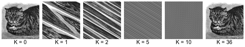
The minimum recurrence time for an image is the minimum positive integer $k \geq 1$ such that $C^k(x, y) = (x, y)$ for all $(x, y)$. In simple terms, the minimum recurrence time is the minimum number of iterations of the cat map that produce the starting image.

For example, the minimum recurrence time for cat1368.pgm of size $1368 \times 1368$ is $36$. As said before, the minimum recurrence time depends on the image size $N$. Unfortunately, no closed formula is known to compute the minimum recurrence time as a function of $N$, although there are results and bounds that apply to specific cases.

You are provided with a serial program that computes the $k$-th iterate of Arnold’s cat map on a square image. The program reads the input from standard input in PGM (Portable GrayMap) format. The results is printed to standard output in PGM format. For example:

applies the cat map $k=100$ times on cat1368.phm and saves the result to cat1368-100.pgm.

To display a PGM image you might need to convert it to a different format, e.g., JPEG. Under Linux you can use convert from the ImageMagick package:

Modify the function cat_map() to make use of shared-memory parallelism using OpenMP. To this aim it is important to know that Arnold’s cat map is invertible: this means that any two different points $(x_1, y_1)$ and $(x_2, y_2)$ are always mapped to different points $(x'_1, y'_1) = C(x_1, y_1)$ and $(x'_2, y'_2) = C(x_2, y_2)$, suggesting that the destination bitmap $P'$ can be filled concurrently without race conditions (however, see below for some caveats).

Suggestions

The provided implementation of function cat_map() is based on the following template:

for (i=0; i<k; i++) {
        for (y=0; y<N; y++) {
                for (x=0; x<N; x++) {
                        (x', y') = C(x, y);
                        P'(x', y') = P(x, y);
                }
        }
        P = P';
}

The two innermost loops build a $P'$ from $P$; the outermost loop applies this transformation $k$ times, using the result of the previous iteration as the source image. Therefore, the outermost loop can not be parallelized due to a loop-carried dependence (the result of an iteration is used as input for the next iteration).

(I suggest to try option 3. Option 2, although formally correct, does not appear to be efficient in practice: why?).

We can apply the loop interchange transformation to rewrite the code above as follows:

for (y=0; y<N; y++) {
        for (x=0; x<N; x++) {
                xcur = x; ycur = y;
                for (i=0; i<k; i++) {
                        (xnext, ynext) = C(xcur, ycur);
                        xcur = xnext;
                        ycur = ynext;
                }
                P'(xnext, ynext) = P(x, y)
        }
}

This version can be understood as follows: the two outermost loops iterate over all pixels $(x, y)$. For each pixel, the innermost loop computes the target position $(\mathit{xnext}, \mathit{ynext}) = C^k(x,y)$ that the pixel of coordinates $(x, y)$ will occupy after $k$ iterations of the cat map.

Interestingly, this does not appear to be the case (at least, not on every processor). Table 1 shows the execution time of the two versions of the cat_map() function (“Noi loop interchange” refers to option (3) above; “Loop interchange” refers to option (c)). The program has been compiled with:

(-O0 prevents the compiler to make code transformations that might alter significantly our functions) and executed with the command line:

On some platforms (Intel i5, i7 and Raspberry Pi 4) there is essentially no difference between the two versions. Loop interchange provides a significant performance boost on the very old Atom N570. On the other hand, loop interchange provides worse performance on the Xeon processors.

To probe further

Table 1: Execution time (in seconds) of different implementations.
Processor type	Cores	GHz	GCC version	No loop interchange	Loop interchange
Intel Xeon E3-1220	4	3.5	7.5.0	7.10	12.94
Intel Xeon E5-2603	12	1.7	9.4.0	5.94	7.53
Intel i7-4790	4+4	3.6	7.5.0	6.01	5.92
Intel i5-11320H	4+4	4.5	9.4.0	3.94	4.01
Intel Atom N570	2+2	1.6	7.5.0	128.69	92.47
Raspberry Pi 4	4	1.5	8.3.0	27.10	27.24

What is the minimum recurrence time of image cat1024.pgm of size $1024 \times 1024$? Since there is no general formula, to answer this question we need to iterate the cat map and stop as soon as we get an image that is equal to the original one.

It turns out that there is a smarter way, that does not involve slow comparisons of images. There is actually no need to have an input image at all: only its size $N$ is required.

To see how it works, let us suppose that we know that one particular pixel of the image, say $(x_1, y_1)$, has minimum recurrence time equal to 15. This means that after 15 iterations of the cat map, the pixel at coordinates $(x_1, y_1)$ will return to its starting position.

Suppose that another pixel of coordinates $(x_2, y_2)$ has minimum recurrence time 21. How many iterations of the cat map are required to have both pixels back to their original positions?

The answer is $105$, which is the least common multiple (LCM) of 15 and 21. From this observation we can devise the following algorithmn for computing the minimum recurrence time of an image of size $N \times N$. Let $T(x,y)$ be the minimum recurrence time of the pixel of coordinates $(x, y)$, $0 \leq x, y < N$. Then, the minimum recurrence time of the whole image is the least common multiple of all $T(x, y)$.

omp-cat-map-rectime.c contains an incomplete skeleton of a program that computes the minimum recurrence time of a square image of size $N \times N$. A function that computes the LCM of two positive integers is provided therein. Complete the program and then produce a parallel version using the appropriate OpenMP directives.

Table 2: Minimum recurrence time for some image sizes \(N\)
\(N\)	Minimum recurrence time
64	48
128	96
256	192
512	384
1368	36

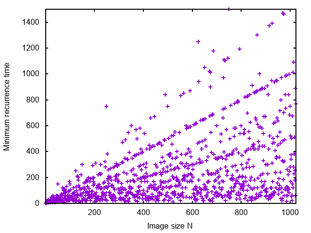
Figure 3 shows the minimum recurrence time as a function of $N$. Despite the fact that the values “jump” from size to size, we see that they tend to align along straight lines.

Suggestions

To probe further

Files