HPC - Rule 30 Cellular Automaton

We introduced Cellular Automata (CAs) as an example of stencil computations. In this exercise we implement the Rule 30 Cellular Automaton.

The Rule 30 CA is a 1D cellular aotmaton that consists of an array x[N] of \(N\) integers that can be either 0 or 1. The state of the CA evolves at discrete time steps: the new state of a cell depends on its current state, and on the current state of the two neighbors. We assume cyclic boundary conditions, so that the neighbors of \(x[0]\) are \(x[N-1]\) and \(x[1]\) and the neighbors of \(x[N-1]\) are \(x[N-2]\) and \(x[0]\) (Figure 1).

Given the current values \(pqr\) of three adjacent cells, the new value \(q'\) of the middle cell is computed according to Table 1.

The sequence □□□■■■■□ = 00011110 on the second row is the binary representation of decimal 30, from which the name (“Rule 30 CA”); more details can be found here.

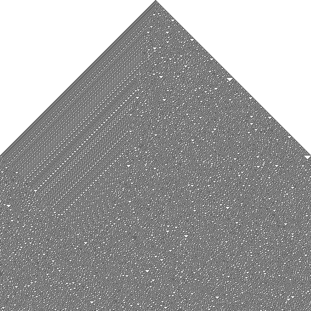
The file mpi-rule30.c contains a serial program that computes the evolution of the Rule 30 CA, assuming an initial condition where all cells are 0 except the central one. The program accepts two optional command line parameters: the domain size \(N\) and the number of steps nsteps to simulate. At the end, process 0 produces the image rule30.pbm shown in Figure 2 of size \(N \times \textit{nsteps}\).

Each row of the image represents the state of the automaton at a specific time step (1 = black, 0 = white). Time moves from top to bottom: the first line is the initial state (time 0), the second line is the state at time 1, and so on.

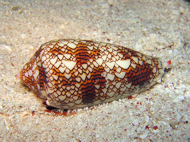
Interestingly, the pattern shown in Figure 2 is similar to the pattern on the Conus textile shell, a highly poisonous marine mollusk which can be found in tropical seas (Figure 3).

The goal of this exercise is to parallelize the serial program using MPI, so that the computation of each step is distributed across the MPI processes. The program should operate as follows (see Figure 4):

1. The domain is distributed across the \(P\) MPI processes using MPI_Scatter() (assume that \(N\) is a multiple of \(P\)). Each partition is augmented with two ghost cells that are required to compute the next states.

2. Each process sends the values on the border of its partition to the neighbors using MPI_Sendrecv(). This operation must be performed twice, to fill the left and right ghost cells (see below).

3. Each process computes the next state for the cells in its partition.

4. Since we want to dump the state after each step, the master collects all updated partitions using MPI_Gather(), and stores the resulting row to the output file.

At the end of step 4 we go back to step 2: since each process already has its own updated partition, there is no need to perform a new MPI_Scatter() every time.

Let comm_sz be the number of MPI processes. Each partition at step 1 has (\(\mathit{local\_width} = N / \mathit{comm\_sz} + 2\)) elements (including the ghosts cell). We denote with cur[] the complete domain stored on process 0, and with local_cur[] the partitions assigned to each process.

Assuming that cur[] is also extended with two ghost cells, as in the program provided (this is not required in the MPI version), the distribution of cur[] can be accomplished with the instruction:

MPI_Scatter( &cur[LEFT],        /* sendbuf    */
             N/comm_sz,         /* Sendcount  */
             MPI_INT,           /* sendtype   */
             &local_cur[LOCAL_LEFT],/* recvbuf    */
             N/comm_sz,         /* recvcount  */
             MPI_INT,           /* recvtype   */
             0,                 /* root       */
             MPI_COMM_WORLD     /* comm       */
             );

(the symbols LEFT and LOCAL_LEFT are defined in the source code to improve readability).

Filling the ghost cells is a bit tricky and requires two calls to MPI_Sendrecv() (see Figure 5). First, each process sends the value of the rightmost domain cell to the successor, and receives the value of the left ghost cells from the predecessor. Then, each process sends the contents of the leftmost cell to the predecessr, and receives the value of the right ghost cell from the successor. All processes execute the exact same type of communication: therefore, each one should call MPI_Sendrecv() twice in the same way (possibly with different parameters).

To compile:

    mpicc -std=c99 -Wall -Wpedantic mpi-rule30.c -o mpi-rule30

To execute:

    mpirun -n P ./mpi-rule30 [width [steps]]

Example:

    mpirun -n 4 ./mpi-rule30 1024 1024

The output is stored to a file rule30.pbm

Files

• mpi-rule30.c
• Additional information