Last updated: 2023-06-07
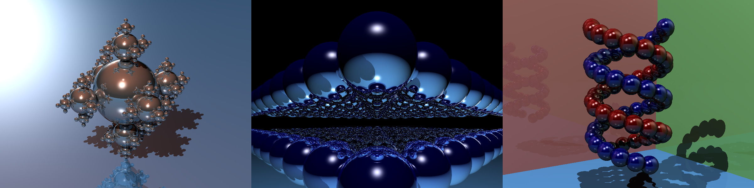
The file omp-c-ray.c contains the implementation of a simple ray tracer written by John Tsiombikas and released under the GPLv2+ license. Figure 1 shows a few images that can be produced by this program.
Table 1 shows the approximate rendering time of each image on the lab machine (Xeon E5-2603 1.70GHz), using a single core.
| File | Time (s) |
|---|---|
| sphfract.big.in | 895.5 |
| sphfract.small.in | 36.5 |
| spheres.in | 27.9 |
| dna.in | 17.8 |
The goal of this exercise is to parallelize the render() function using OpenMP. The serial program is well structured: functions don’t modify global variables, so there are not hidden dependences. If you have time, measure the speedup and the strong scaling efficienty of the parallel version.
Although not strictly necessary, it is useful to know how a ray tracer works using Whitted recursive algorithm (Figure 2).

The scene is represented by a set of geometric primitives (spheres, in our case). We generate a primary ray (V) from the observer towards each pixel. For each ray, we determine the intersections with the spheres in the scene, if any. The intersection point p that is closest to the observer is selected, and one or more secondary rays are cast, depending on the material of the object p belongs to:
A light ray (L) towards each light source, to see whether p is directly illuminated.
If the surface is reflective, we generate a reflected ray (R) and repeat the procedure recursively.
If the surface is translucent, we generate a transmitted ray (T) and repeat the procedure recursively (omp-c-ray does not support translucent objects, so this never happens).
The time required to compute the color of a pixel depends on the number of spheres and lights in the scene, and on the material of the spheres; reflective or translucent surfaces produce additional rays that must be handled. This suggests that the time required to compute the color of each pixel is highly variable, which leads to load imbalance.
To compile:
gcc -std=c99 -Wall -Wpedantic -fopenmp omp-c-ray.c -o omp-c-ray -lmTo render the scene sphfract.small.in:
./omp-c-ray -s 800x600 < sphfract.small.in > img.ppmThe command above produces an image img.ppm with a resolution \(800 \times 600\). To view the image on Windows it is useful to convert it to JPEG format using the command:
convert img.ppm img.jpegand then transferring img.jpeg to your PC for viewing.
The omp-c-ray program accepts a number of optional command-line parameters; to see the complete list, use
./omp-c-ray -h